FDPNP8: Inside the Vision Transformer (Part 1)
Preface: I want to initiate a comprehensive series, “Fundamentals of Digital Pathology for Novice Pathologists (FDPNP)”. This endeavor aims to disseminate knowledge about the utilization of computer vision in the realm of modern pathology to pathologists who want to know more about digital pathology.
Introduction
We continue our journey in exploring the Vision Transformer (ViT). It is possible to utilize both transformer and convolutional modules in a deep learning model. However, the original authors of ViT demonstrated that convolutional layers aren’t necessary for processing images within the ViT model [1], thereby making it a unique method for handling visual data. The architecture of ViT draws inspiration from the language transformer model presented in the seminal paper, “Attention is All You Need” [2].
Before we delve into the workings of the Vision Transformer (ViT), it’s crucial to grasp the concept of the attention mechanism within the realm of deep learning.
Inside the attention
The concept of attention, while crucial, can be intricate to encapsulate succinctly. Thus, we’ll explore attention through a straightforward example. If you recall from FDPNP1, we introduced the idea of a hand matrix. Now, let’s assume we wish to decompose this hand matrix into five vectors, with each vector representing a finger of the hand.
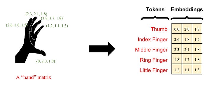
Image by Author
Each finger can be characterized by the lengths of its individual phalanges, forming a three-dimensional vector. In a more comprehensive context, each finger can be viewed as a token. We refer to this vector as the ‘embedding’ of a finger. The hand comprises five fingers, each of which can be represented by its unique embedding. Now, let’s explore how the attention mechanism operates on this hand input.
Firstly, we adjust the dimensions of these five embeddings. We utilize a fully connected (FC) layer to project the three-dimensional embeddings into higher-dimensional vectors, say, 64 dimensions. This process is known as the creation of the hidden dimension.
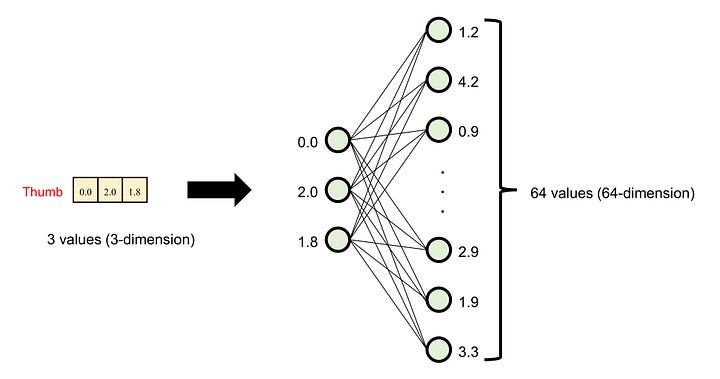
Image by Author
In the attention mechanism, this projection is performed thrice, each time with a different FC layer. These layers are referred to as the key (FCk), query (FCq), and value (FCv) FC layers. Consequently, a finger (a token) embedding yields three 64-dimensional embeddings: key, query, and value (KQV). Essentially, when we input the hand matrix, we obtain the key, query, and value matrices, each of which has 5 rows and 64 columns.
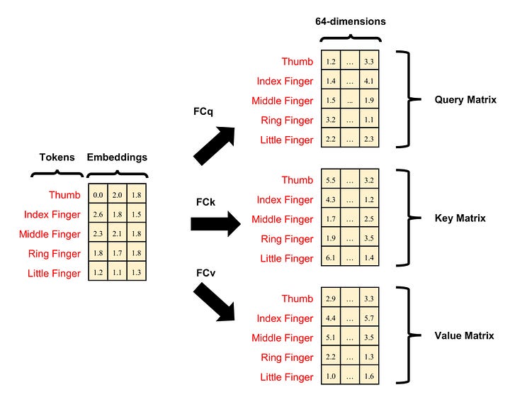
Image by Author
Next, we compute the attention scores, which are the resulting products of the query and transposed key matrices.
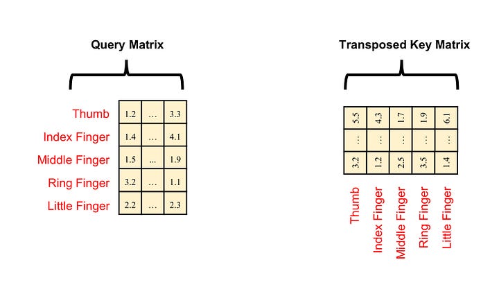
Image by Author
These scores are represented as a matrix. I will break down the steps of calculation. First, we calculate the dot products of each row of query (each finger/token) and each column of transposed key (each finger/token). Here is how the operation works:
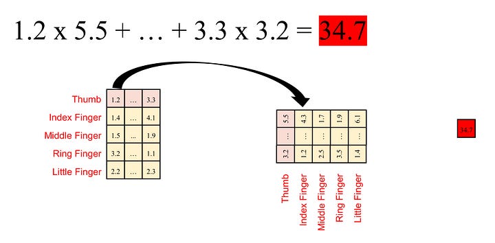
Image by Author
We calculate the multiplication of each element in an embedding of the query matrix with each corresponding element in an embedding of the key matrix and then sum them up. For instance, for embedding Q (q1, …, q64) from the query and embedding K (k1, …, k64) from the key, we compute the dot product value (k1q1 + … + k64q64). Each embedding in the query matrix results in five dot product values (since we have five embeddings in the key matrix in our example). This gives us a total of 25 dot product values, arranged in the form of a 5x5 matrix, called the attention mask.
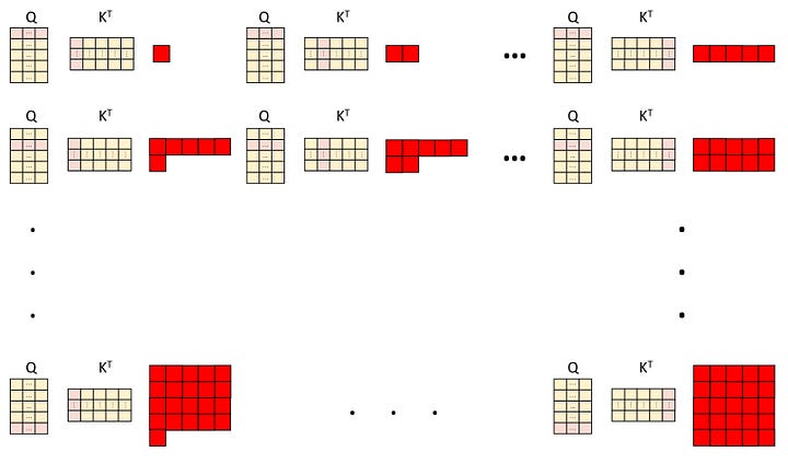
Image by Author
Next, we apply the 1-dimensional Softmax transformation to each row in this matrix. The total sum of Softmax-transformed values in each row equals one. Each row corresponds to a specific finger/token. Each cell in this row represents the attention score of that specific finger/token in relation to each of the five fingers/tokens, including itself.
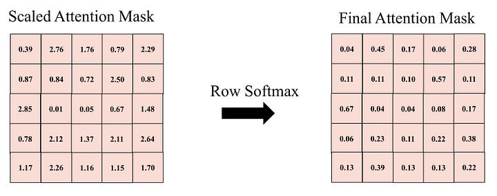
Image by Author
In the end, we construct the final matrix by multiplying the attention mask with the value matrix. This involves performing a multiplication operation for each row of the attention mask (which corresponds to a token) and each column of the value matrix, and summing the results to obtain a single value. This procedure is executed 64 times for each column, generating 64 values for the first row. We then advance to the next row of the attention mask and repeat the same operation. The resulting matrix comprises 5 rows and 64 columns.
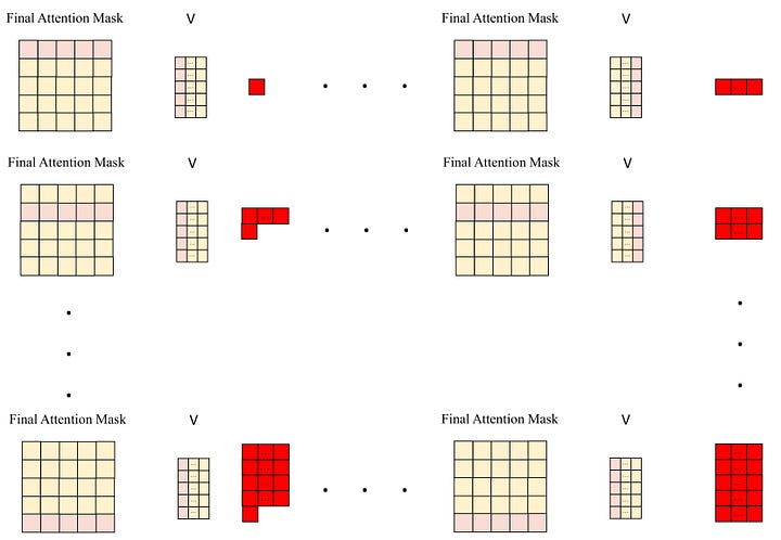
Image by Author
In summary, we start with an input known as a ‘hand matrix’, which comprises 5 rows (symbolizing 5 ‘fingers’ or tokens) and 3 columns (representing the raw embeddings). This matrix is transformed into an output referred to as a ‘hand-attended’ matrix, which consists of 5 rows (corresponding to the 5 tokens) and 64 columns (representing the attended embeddings). This output matrix captures the intricate relationships among the 5 tokens/fingers, which are established through numerous integration processes involving matrix multiplication.
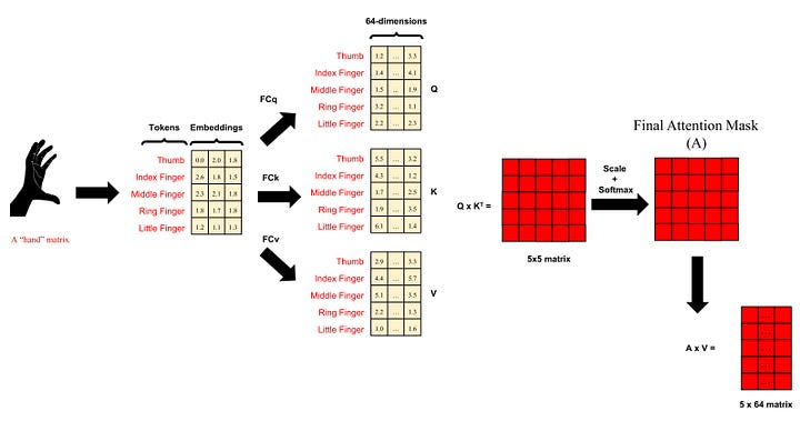
Image by Author
Multi-head Attention
Consider a scenario where we project three-dimensional finger embeddings into 16 dimensions. The twist is that we perform this operation 4 times, each with a different set of KQV triads. Each of these triads independently undergoes the attention operation. The resulting matrices each consist of 5 rows (representing 5 fingers) and 16 columns (representing attended embeddings). We then assemble all these final matrices together by concatenating them column-wise. This is what we mean when we say the attention mechanism has 4 heads or multi-head attention.
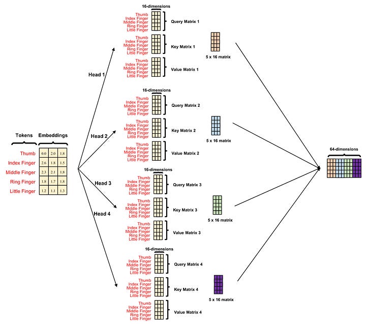
Image by Author
Conclusion
The attention operation forms the bedrock of the Transformer module, a crucial component of the Vision Transformer. However, comprehending this operation necessitates a solid understanding of matrix multiplication, which I tried to describe in full detail in this blog.
To those who may be interested, I hope you enjoy this mini-review.
References
-
Vaswani, Ashish, et al. “Attention Is All You Need.” ArXiv.org, 12 June 2017, arxiv.org/abs/1706.03762.
-
Dosovitskiy, Alexey, et al. “An Image Is Worth 16x16 Words: Transformers for Image Recognition at Scale.” ArXiv:2010.11929 [Cs], 22 Oct. 2020.