FDPNP9: Inside the Vision Transformer (Part 2)
Preface: I want to initiate a comprehensive series, “Fundamentals of Digital Pathology for Novice Pathologists (FDPNP)”. This endeavor aims to disseminate knowledge about the utilization of computer vision in the realm of modern pathology to pathologists who want to know more about digital pathology.
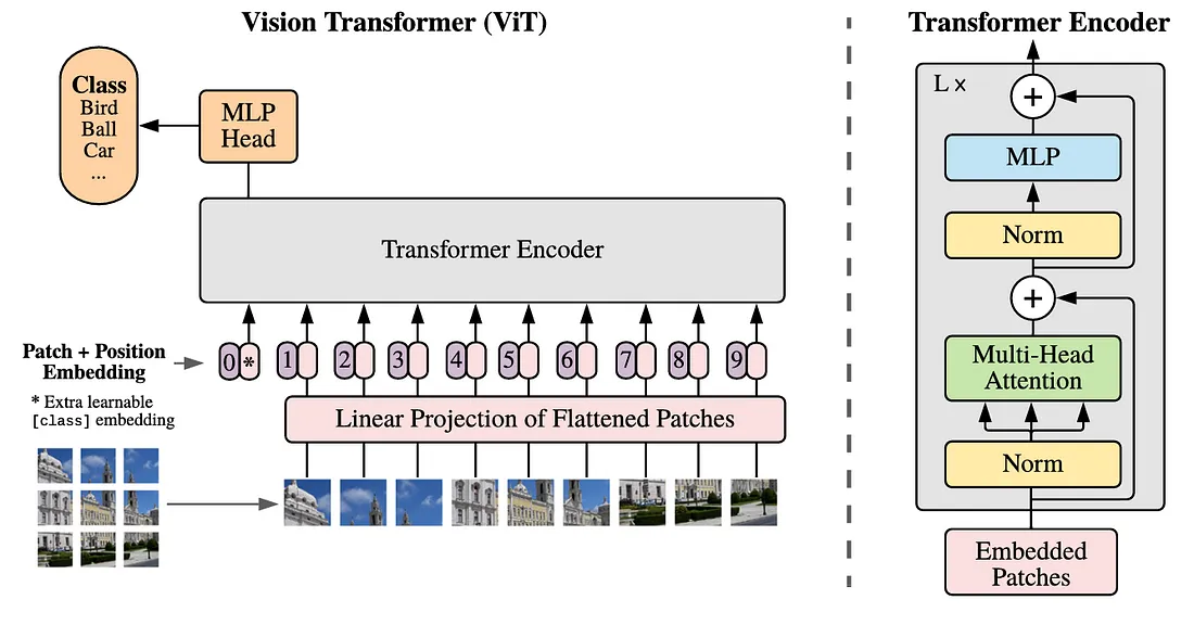
Image by Original Paper [1]
Image Tokenization and Embedding
In FDPNP8, we briefly touched upon the concept of a token. A token is equivalent to a finger in our previous example or a word in the realm of natural language processing. It’s possible to embed a token into a vector. However, an image, being a 3D tensor, doesn’t neatly fit into the concept of a vector. Therefore, it’s crucial to understand how to transform an image into multiple tokens. This procedure is known as image tokenization.
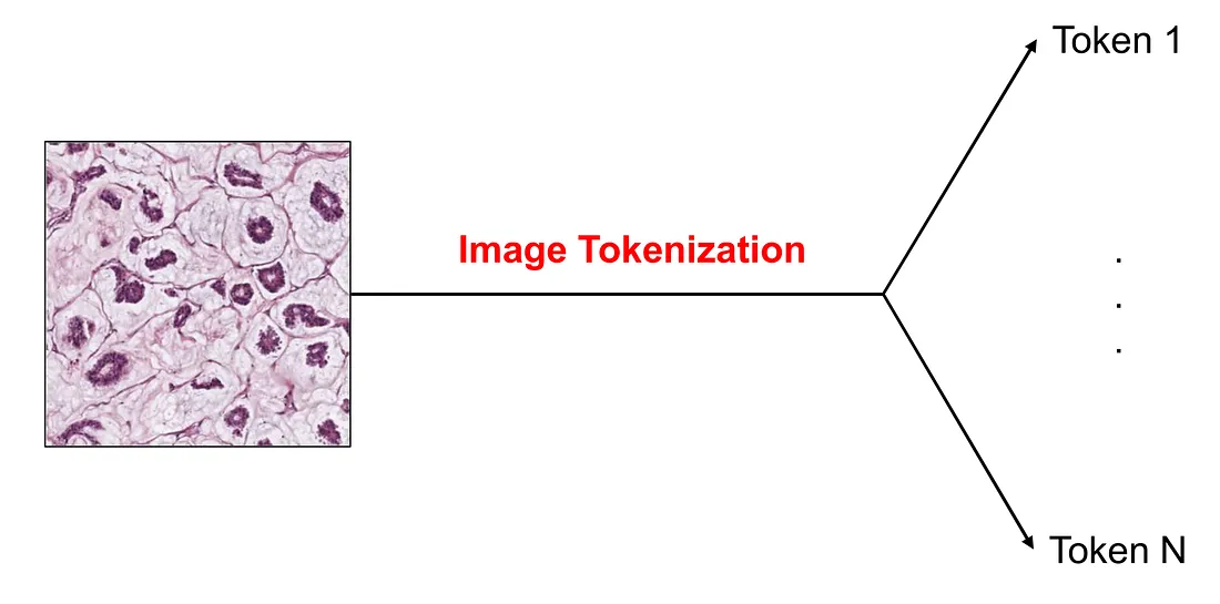
Image by Author
In the Vision Transformer (ViT) model, the input image is initially divided into small, square patches that do not overlap. Each of these patches is subsequently flattened into a vector. For instance, if a patch measures 16 x 16, its shape would be 3 x 16 x 16, where 3 represents the number of color channels. The result of this flattening process is a vector with 768 dimensions.
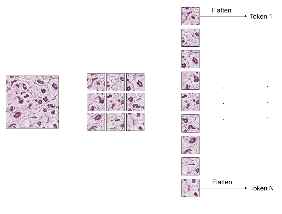
Image by Author
In summary, we start with an image. The end result is a series of 768-dimensional vectors. The image can be likened to a hand, and each of these vectors to a finger. However, unlike our previous example which had 3 dimensions, each vector in this case has 768 dimensions.
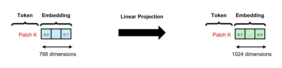
Image by Author
The next step is to create a patch embedding. We project the 768-dimensional vectors created by the flattening process to 1024-dimensional vectors by using a fully-connected layer. This process is called linear projection.
The Classification Token
Before we put all the tokens into the ViT, we artificially create another token at the beginning of the token sequence, namely the classification token. This token is important since its corresponding final embedding is used for the classification task.
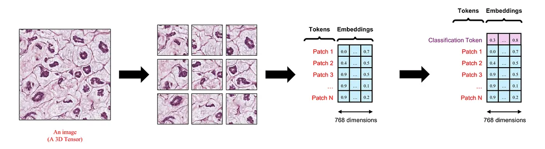
Image by Author
Inside the Vision Transformer
If the input image has a size of 224 x 224 pixels, it can be segmented into 196 small square patches, each measuring 16 x 16 pixels, we collect 196 tokens, each possessing 768 dimensions, for each image via image tokenization. These 196 tokens are subsequently projected into 196 hidden embeddings, each encompassing 1024 dimensions.
Image by Original Paper [1]
After creating the patch embeddings, we project these embeddings into key, query, and value vectors for the multi-head attention mechanism. The final results are 196 first-time attended vectors, each representing the corresponding token.
In ViT, these vectors can go through multiple layers of the attention mechanism, depending on the size of the model. The number of layers (L) can be 12, 24, or 36.
Positional Embedding
Positional Embedding is a well-established technique used to incorporate the position information of tokens. Each token’s initial embedding is enhanced with its corresponding positional embedding before being processed through the layers of the transformer block. The creation of this embedding, however, falls outside the purview of this blog post.
Conclusion
ViT represents a class of computer vision models that do not contain convolutional operations. The transformer layers within ViT are fundamentally predicated on the attention mechanism. In practice, it’s possible to construct hybrid models that incorporate both transformer and convolutional modules.
To those who may be interested, I hope you enjoy this mini-review.
Reference
- Dosovitskiy, Alexey, et al. “An Image Is Worth 16x16 Words: Transformers for Image Recognition at Scale.” ArXiv:2010.11929 [Cs], 22 Oct. 2020.