FDPNP7: Inside the Convolution
Preface: I want to initiate a comprehensive series, “Fundamentals of Digital Pathology for Novice Pathologists (FDPNP)”. This endeavor aims to disseminate knowledge about the utilization of computer vision in the realm of modern pathology to pathologists who want to know more about digital pathology.
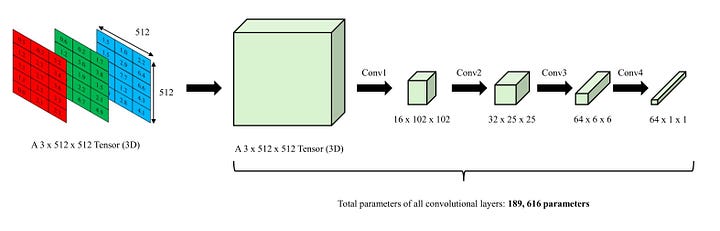
Image by Author
Introduction
In FDPNP1, we discussed how computers perceive images [1]. An image is viewed as a 3D tensor, comprising three matrices that correspond to the Red, Green, and Blue (RGB) colors. Each matrix value plays a role in forming the color of a specific pixel, in conjunction with its equivalent values in the other two matrices. These three corresponding values, also known as color channels, collectively encode a single-color pixel.
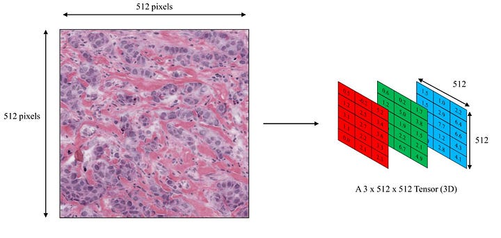
Image by Author
In our previous blogs, we delved into the workings of an Artificial Neural Network (ANN) and its components, the artificial neurons [2, 3]. An ANN that has more than two hidden layers is classified as a deep learning model. Conventionally, these models are adept at handling a vector of numbers within their internal mechanisms. However, when we apply the procedures discussed in FDPNP5 and FDPNP6 to work with tensor or matrix inputs, it results in overcomplication due to a massive number of parameters. This is because these operations concentrate on the input as a vector of single values, not a tensor with a higher order. A higher number of parameters also implies a larger set of training samples.
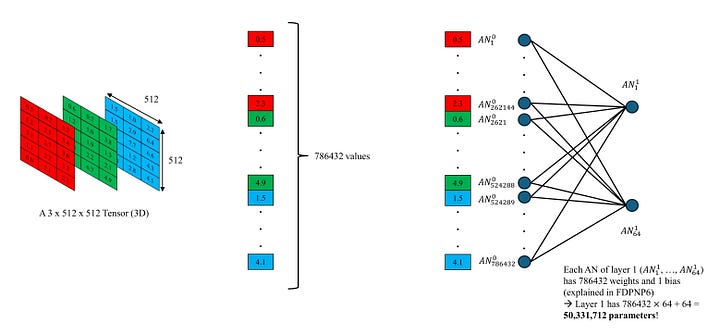
Image by Author
In other words, dealing with matrices and tensors necessitates the use of specific layers or operations. For the sake of simplicity, I will only touch upon the two key operations: convolution and attention-based vision transformers. The performance of deep convolutional neural networks (DCNN) and transformer-based networks is comparable. The superiority of one over another depends on the task at hand. They are all state-of-the-art computer vision models. In this blog, I only focus on convolution and reserve the vision transformer for the next blog (FDPNP8).
Number of parameters in an example of convolutions - Image by Author
Inside the Convolution
To simplify, my focus will be on 2D convolution, as it is frequently employed in digital and computational pathology. However, the mechanisms of 1D and 3D convolutions are identical. In a convolution operation, there are units known as filters or kernels. Each of these is essentially a small 3D tensor. The size and quantity of these tensors are user-determined.
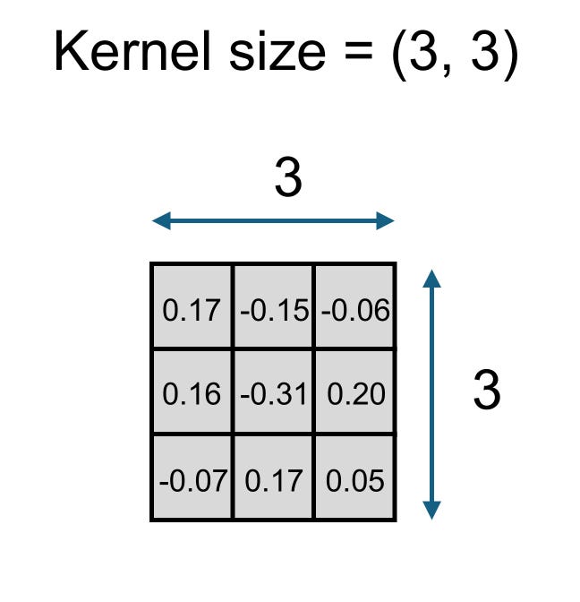
A 2D kernel - Image by Author
To give a sense of how each kernel works, imagine we have two 3 x 3 matrices of identical size. One is referred to as the input matrix, while the other is the kernel. The input matrix contains 9 input values, and the kernel also houses 9 values, known as weights. This kernel operates on the input matrix by multiplying its weights with the corresponding input values and then summing them all. The end result is a singular value.
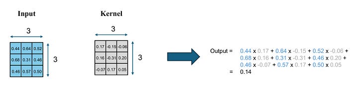
Image by Author
Let’s assume we have a different input matrix and the same kernel. The kernel processes in an identical manner, but it produces a distinct output because the two input matrices are not the same.
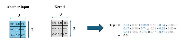
Image by Author
When the kernel is a 3 x 3 matrix, we refer to the kernel size as (3, 3). Besides filters or kernels, convolutions possess additional features that require user decisions, such as input channels, output channels, and stride.
To illustrate the concept of input and output channels, let’s revisit the previous example of one kernel processing one input. Suppose we have a combined input from the two aforementioned input matrices. Consequently, our input and kernel become 3D tensors (2, 3, 3). Recall that a tensor is a generalized form of a matrix [1].
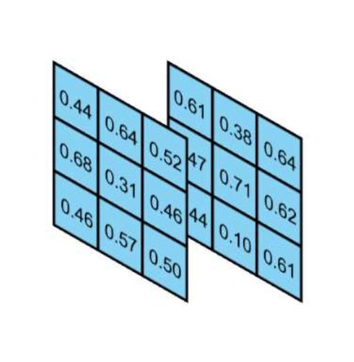
Image by Author
The kernel processes the input tensor matrix by matrix, generating two output values. These values are subsequently added together to yield the final result, a singular value. When the input is a 3D tensor of (N, 3, 3), the kernel tensor is also (N, 3, 3), and we refer to N as the number of input channels. In our example, we have 2 input channels.
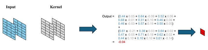
Image by Author
Now, imagine we augment the number of kernels to three. We now possess three kernel tensors with the size of 2 x 3 x 3, while maintaining the input as a (2, 3, 3) tensor. This input will sequentially pass through each kernel in the same manner, generating three final outputs. Consequently, we end up with an output comprising three values.
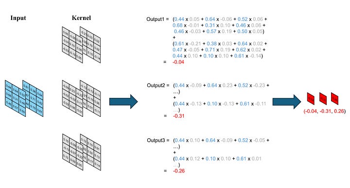
Image by Author
Note that the number of outputs generated each time a kernel computation is performed equates to the number of output channels.
Number of kernels = Number of outputs for each kernel computation = Number of output channels
Now, let’s turn our attention to the concept of stride. First of all, we enlarge our 3D input tensor to a (2, 5, 5) tensor, while maintaining the size and number of kernels unchanged.
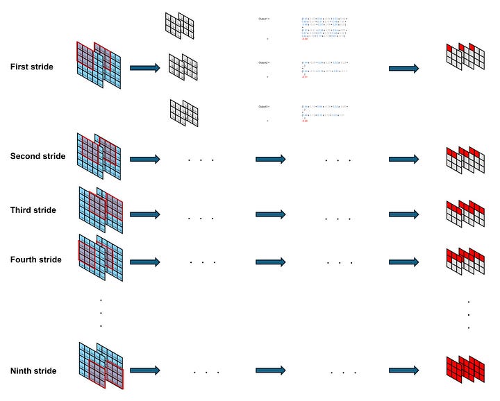
Image by Author
Given that the kernel size is smaller than the dimensions of the input tensor, the kernels traverse across the columns and rows similar to sliding windows. The stride dictates the pace at which they advance during each computation.
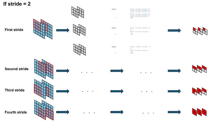
Image by Author
It is important to note that the output of this convolution is also a 3D tensor. The depth dimension of this tensor corresponds to the number of kernels. The dimensions of width and height depend on the magnitude of the stride.
Finally, we also introduce biases in convolution. These biases are incorporated after computing the output for each channel. Consequently, the quantity of biases aligns with the number of kernels.
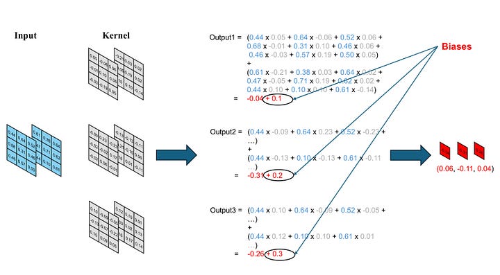
Image by Author
Each component of a convolution operation is referred to as a filter or a kernel, which is essentially a 3D tensor populated with weights. The basic attributes of a convolution include the kernel size, input channels, output channels, and stride. Biases are added to each output channel.
There are also additional advanced attributes such as padding, input-output connection, or dilation. For the purpose of understanding, we do not cover these arguments.
2D Convolution to Handle an Image
Suppose we have a small color image from histopathology that is 10 x 10 pixels. As we know, this image can be represented as a 3D tensor of dimensions 3 x 10 x 10 [1]. We will process this image using three convolution operations:
-
The first convolution (conv1): a kernel size of (3, 3), input channels of 3, output channels of 8, and a stride of 2.
-
The second convolution (conv2): a kernel size of (2, 2), input channels of 8, output channels of 32, and a stride of 1.
-
The final convolution (conv3): a kernel size of (3, 3), input channels of 32, output channels of 64, and a stride of 1.
In conv1, we have eight kernels, each of size 3 x 3. Each kernel interacts with all the channels in the windowed portion of the input to produce a single output value. As a result, each windowed portion of the input generates 8 channels of a value in Output 1. By moving this window 2 pixels at a time (stride = 2), we create an Output 1 tensor of dimensions 8 x 4 x 4.
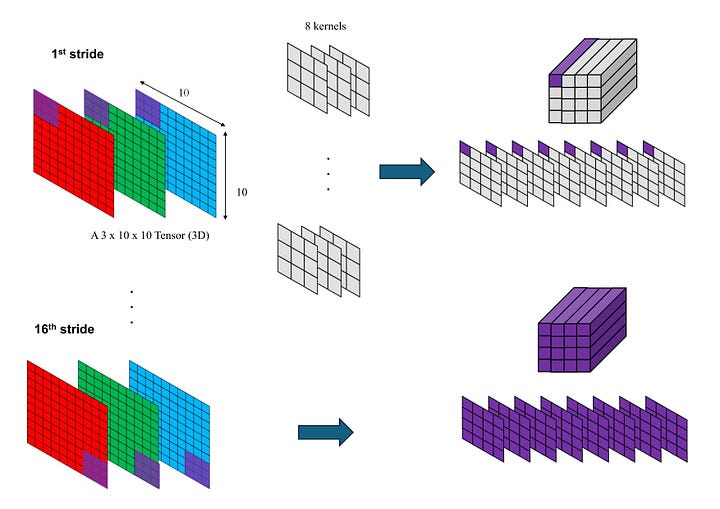
Image by Author
In conv2, we utilize 32 kernels, each of size 2 x 2. Following the same logic, each windowed portion of Output 2 generates 32 channels of a value in Output 2. By shifting this window one value at a time (stride = 1), we construct an Output 2 tensor of dimensions 32 x 3 x 3.
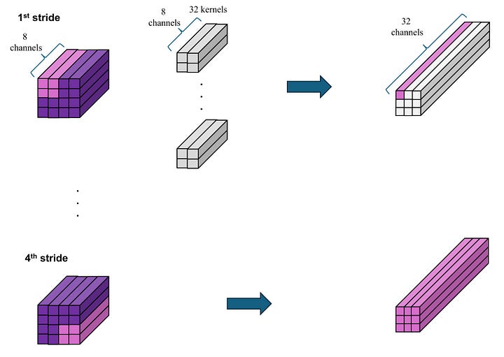
Image by Author
In a manner similar to conv3, we obtain an Output 3 tensor of dimensions 64 x 1 x 1.
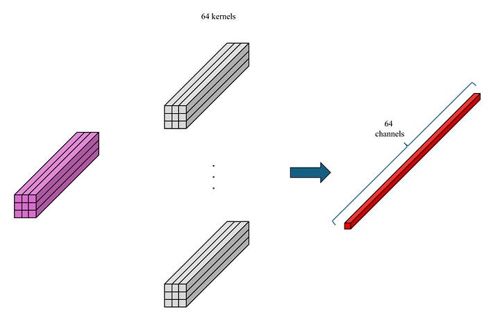
Image by Author
Outputs 1, 2, and 3 are referred to as feature maps or activation maps.
The intermediate tensors that act as the output of the preceding convolutional layer and the input of the subsequent convolutional layer are termed feature maps or activation maps.
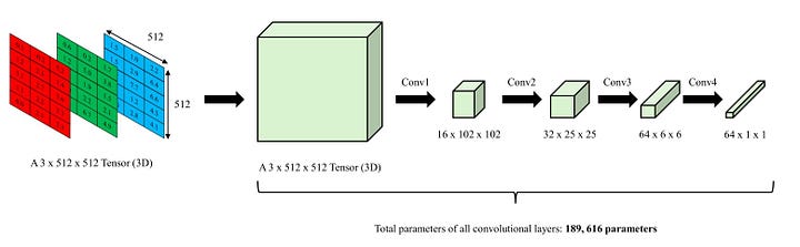
The total number of weights of these 3 convolutional layers is 19,672.
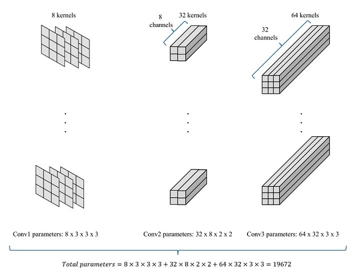
Image by Author
Why Convolutions?
Among many reasons, I found two significant ones: Translational Invariance and Parameter Sharing.
Translational invariance refers to the ability to recognize the local “visual structure” information, as each convolution computes the value locally based on the kernel size. That means it does not matter where a small object is located in the picture. The convolutions can still find out.
Parameter Sharing refers to the use of the same kernels across each sliding window. For instance, the first convolutional layer (conv1) uses the same 8 kernels as it scans a 10 x 10 image. This means that conv1 does not use different kernels (and thus, weights) for each sliding window. This significantly reduces the number of parameters, thereby mitigating the problem of overcomputation. While this issue may not be apparent with small-sized images, it becomes substantial when we scale up the image to realistic sizes such as 128 x 128, 256 x 256, 512 x 512, and so on.
In the case of 512 x 512 images, a classic Artificial Neural Network (ANN) model would need to contain at least 402,653,184 weights to convert them into 512-dimensional vectors. However, with a properly designed convolutional model, this number may be reduced to about a few million weights. This represents a significant decrease in parameters.
We can see it in this simple example:
import torch
import torch.nn as nn

# Create an object x of a 512 x 512 image
x = torch.rand(1, 3, 512, 512)

# Classic ANN model
lin = nn.Sequential(
    nn.Flatten(),
    nn.Linear(512*512*3, 512, bias=False)
)

# Convolutional model
convolutions = nn.Sequential(
    nn.Conv2d(in_channels=3, out_channels=8, kernel_size=3, stride=2, bias=False),
    nn.Conv2d(in_channels=8, out_channels=32, kernel_size=3, stride=3, bias=False),
    nn.Conv2d(in_channels=32, out_channels=64, kernel_size=3, stride=3, bias=False),
    nn.Conv2d(in_channels=64, out_channels=128, kernel_size=3, stride=3, bias=False),
    nn.Conv2d(in_channels=128, out_channels=256, kernel_size=3, stride=3, bias=False),
    nn.Conv2d(in_channels=256, out_channels=512, kernel_size=3, stride=2, bias=False),
    nn.Flatten()
)

print(f"Output size of classic ANN model: {lin(x).shape[1]}")
print(f"Output size of convolutional model: {convolutions(x).shape[1]}")
print(f"Weights of classic ANN model: {sum(p.numel() for p in lin.parameters())}")
print(f"Weights of convolutional model: {sum(p.numel() for p in convolutions.parameters())}")

# This is the output:
Output size of classic ANN model: 512
Output size of convolutional model: 512
Weights of classic ANN model: 402653184
Weights of convolutional model: 1569240
In summary, convolutions are advantageous for image processing because they (1) recognize the local visual information of the image, and (2) have considerably fewer weights compared to a fully-connected layer.
Conclusion
In computer vision, the convolution layer and vision transformer are the pivotal operations to process images. Convolution functions through a set of kernels that traverse across the two primary dimensions (width and height), thereby diminishing the size of these dimensions while augmenting the size of the third dimension (channels).
To those who may be interested, I hope you enjoy this mini-review. If you want to know more about convolution, there are a lot of fantastic articles such as:
https://towardsdatascience.com/intuitively-understanding-convolutions-for-deep-learning-1f6f42faee1
References
- https://minhkhangle-phd.github.io/2023/12/26/post-12.html
- https://minhkhangle-phd.github.io/2024/01/22/post-17.html
- https://minhkhangle-phd.github.io/2024/01/29/post-18.html