FDPNP6: The operation of neural networks (Part 2)
Preface: I want to initiate a comprehensive series, “Fundamentals of Digital Pathology for Novice Pathologists (FDPNP)”. This endeavor aims to disseminate knowledge about the utilization of computer vision in the realm of modern pathology to pathologists who want to know more about digital pathology.

Image by Author
Introduction
In Part 1, we explored the basic components and concepts in the architecture of an artificial neural network (ANN), including artificial neurons (ANs), layers, and modules. In this part, we focus on how they function together when we provide them with input.
The box problem
To understand the workings of an ANN, it’s beneficial to start with a simple example. Let’s assume we have 1000 boxes, each labeled as either small or large. The challenge is in defining the size, which can be ascertained using the provided data (1000 pre-labeled boxes). We measure the width, length, and height of these boxes and utilize these three measurements to classify the size labels. For example, a box with a width of 3 meters, a length of 3.2 meters, and a height of 5.1 meters is represented as an input with three original features (3.0, 3.2, 5.1). Essentially, each box can be represented by a three-dimensional vector (W, L, H), or the three values W, L, and H.
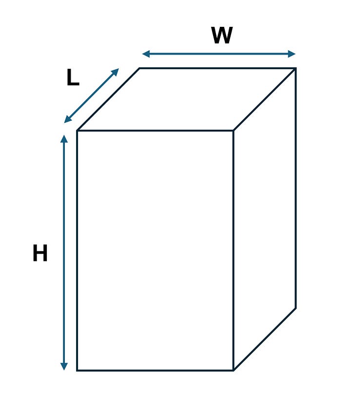
Image by Author
Now that we’ve defined the problem, let’s delve into how an ANN operates. Imagine we construct a simple ANN with an input layer, two hidden layers, and an output layer. The input layer comprises three ANs prepared to receive the values of (W, L, H), while the output layer includes 2 ANs generating probabilities of the box being either small or large. We customize each hidden layer to consist of 2 ANs.
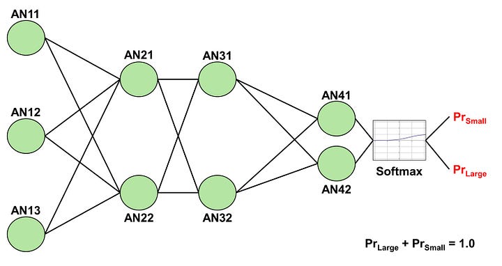
Image by Author
The operation of an AN
Recall that ANs have parameters known as weights and biases. The three input values (W, L, H) = (3.0, 3.2, 5.1) are directed to their corresponding ANs in the input layer: AN11, AN12, and AN13. Each AN in this layer receives an input. A unique aspect of ANs in the input layer is that they do not possess weights and biases; they simply transmit the input to the hidden ANs to which they are connected.
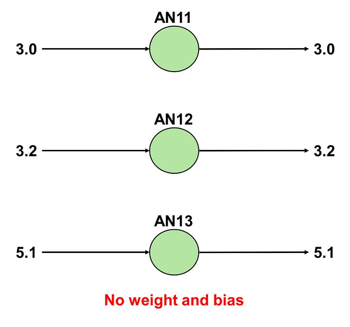
Image by Author
Let us discuss the operation in AN21 and AN22.
AN21 receives three input values from AN11, AN12, and AN13: 3.0, 3.2, and 5.1. Recall that AN has multiple weights to handle multiple inputs. AN21 possesses weights of (0.1, 0.2, 0.3), a bias of 0.2, and employs a ReLU activation function:
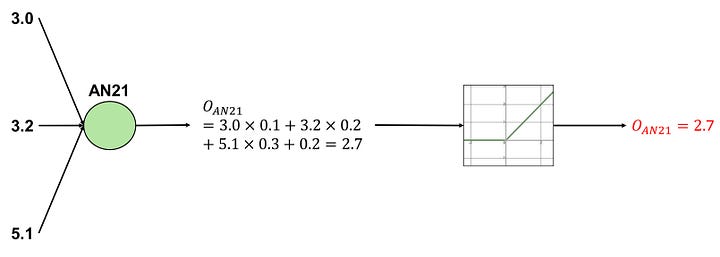
Image by Author
A similar process occurs with AN22. AN22 has weights of (0.5, 0.3, 0.1), a bias of 0.3, and utilizes a ReLU activation function:
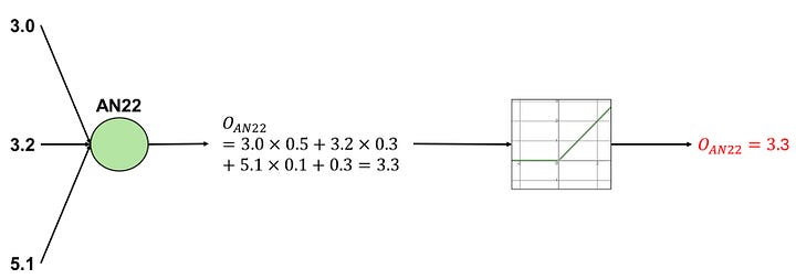
Image by Author
Now, we have the outputs from AN21 and AN22. Since AN31 is connected to both AN21 and AN22, and AN32 is also connected to AN21 and AN22, the outputs from both will be separately delivered to AN31 and AN32.
AN31 has weights of (0.2, 0.2), a bias of 0.2, and employs a ReLU activation function:
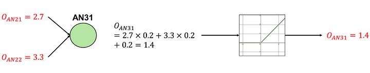
Image by Author
AN32 possesses weights of (0.1, 0.1), a bias of 0.1, and utilizes a ReLU activation function:
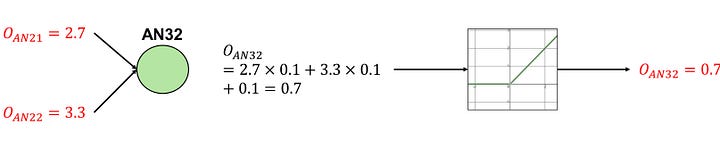
Image by Author
Finally, the outputs from AN31 and AN32 are separately delivered to AN41 and AN42.
AN41 possesses weights of (0.1, 0.2), a bias of 0.3, and employs a Softmax activation function. AN42 has weights of (0.2, 0.3), a bias of 0.4, and also utilizes a Softmax activation function. As the softmax function incorporates both outputs from AN41 and AN42, I will describe these two processes at the same time:
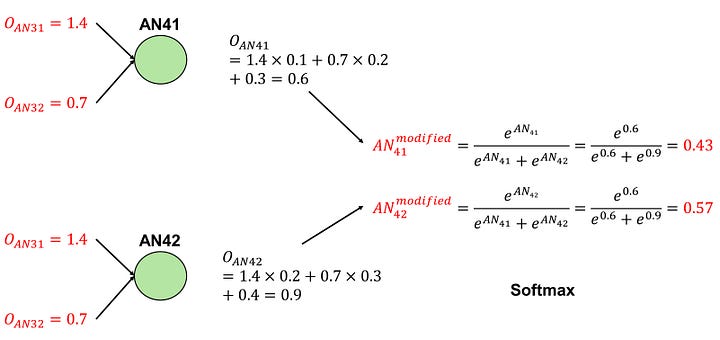
Image by Author
Output Interpretation
The softmax function produces two values, each ranging from 0.0 to 1.0, and their combined sum equals 1.0. As a result, these values can be interpreted as the “relative probabilities” of a box with dimensions (3.0, 3.2, 5.1) being classified as either small or large. In our example, the first value, 0.43, signifies the probability of the box “being small”, while the second value, 0.57, signifies the probability of it “being large”. Given that the probability of the box being large is higher, we can conclude that this ANN categorizes the box as large.
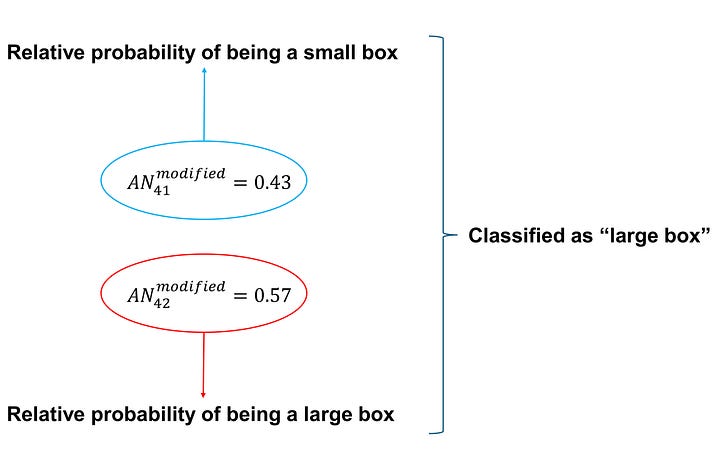
Image by Author
Summary
In essence, the box accepts three inputs: W, L, and H. These inputs are passed on to the ANs of the input layer, specifically AN11-AN13. These ANs, which lack weights, transmit these values to the two hidden neurons (AN21 and AN22) in the next layer. Each of these neurons receives three values and produces a single output, which is then individually sent to each AN (AN31 and AN32) of the subsequent layer. This process is mirrored in these neurons. The outputs from AN31 and AN32 are forwarded to the ANs (AN41 and AN42) of the output layer, which then calculate the relative probabilities of each label, either ‘small’ or ‘large’.
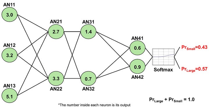
Image by Author
Conclusion
The operation of an ANN is largely governed by the actions of its constituent ANs. The parameters of the AN, its activation function, and the interaction among ANs collectively dictate the output of the ANN.
Having built a solid understanding of how ANNs work, we will next explore the mechanisms of image-processing operations, specifically convolution and attention-based mechanisms, in our upcoming blogs.
To those who may be interested, I hope you enjoy this mini-review.