The Flow of the Data Preparation Process of Histopathology Tasks
In this mini-review, I summarize the data preparation process to create the appropriate data that we can use as histopathological images (patches) and labels to perform a simple task, including regression, classification, segmentation, and self-supervision.
We divide our discussion into 2 parts:
- The data structure of histopathology computer vision (CV) tasks
- The main steps of the data preparation process
The data structure of a histopathology CV task
The two main parts of histopathology CV data are histopathologic slides and clinicopathological metadata.
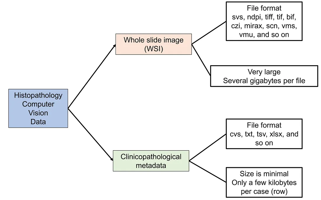
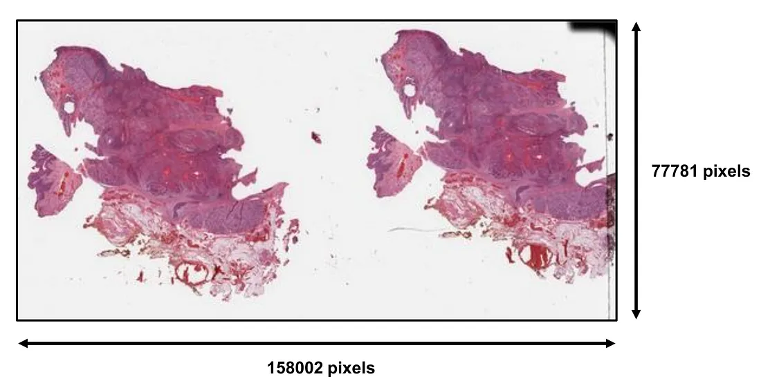
In general, histopathologic slides are saved under the formats of whole slide images (WSI). These WSI files are super-resolution images whose dimensions can be up to thousands to hundreds of thousands of pixels. There is no fixed size of WSI, which depends on the shape and the actual size of the histopathologic slide being saved.
The file types of WSI can be different from scanner to scanner, including svs (Aperio), ndpi, vms, vmu (Hamamatsu), mirax (Zeiss), vms (Ventana), and scn (Leica). The size of each WSI is very large compared to ordinary images. It can range from hundreds of megabytes to gigabytes and terabytes, depending on the dimensions of the WSI.
The clinicopathological metadata is the table containing information about patient ID, different clinical characteristics, and corresponding WSI files.
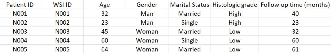
These are the 2 basic components of data structure. However, if we want to perform more advanced tasks such as genetic prediction, or molecular-morphology fusion model, the genetic component can be added to the metadata or a separate file. For example, our task is to predict HER2 amplification using morphology. We would want to incorporate the “HER2 amplification” column into the clinicopathological metadata and use this column to create the label.
The main steps of data preparation
Herein, I list the main steps of data preparation for computer vision tasks in histopathology from my experience. The process can be divided into several basic steps:
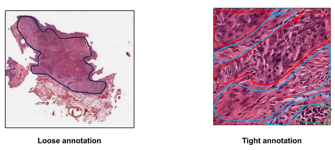
Step 1: WSI annotation. In this step, we have to decide what type of annotation is appropriate to the CV task. For example, a segmentation task requires a “tight” and detailed annotation of the classes being segmented. Say, if we want to construct a segmentation model to classify “tumor”, “stroma”, and “lymphocytes”, the annotator has to tightly mark the area of tumor, stroma, and lymphocytes, even though they are sometimes intertwined together. On the other hand, we may need to only annotate the region of interest (ROI) where the tumor cells reside to pick up the area of the tumor for classification or prognostication tasks.
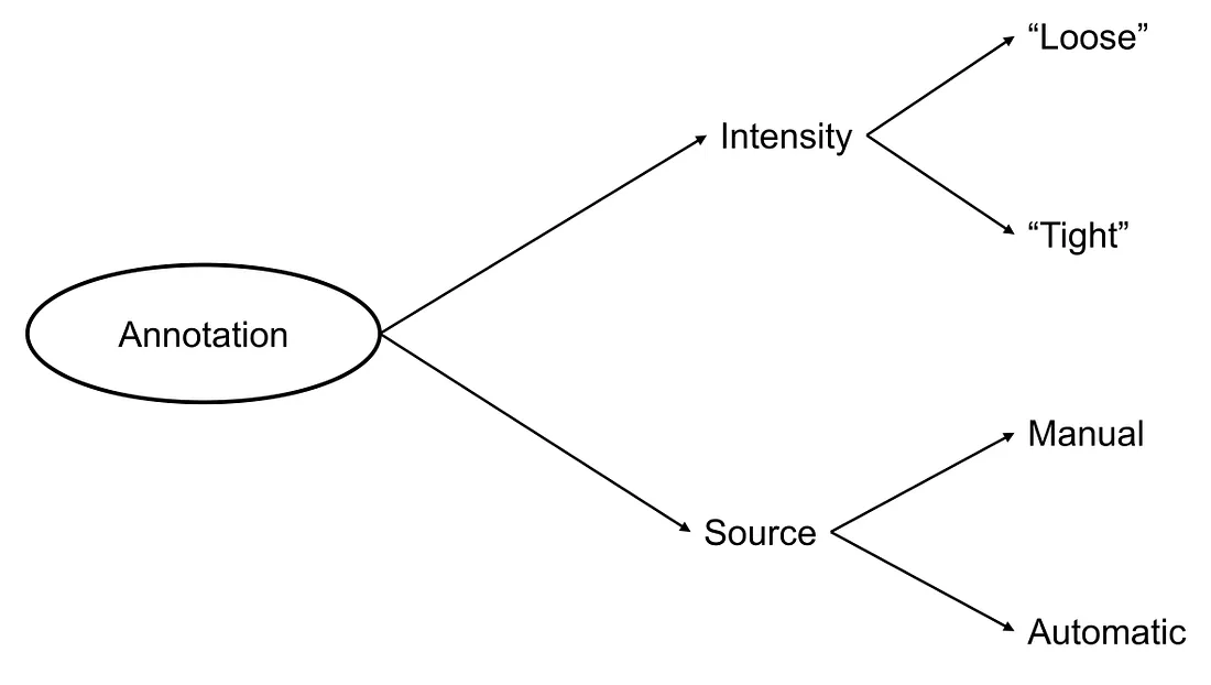
Finally, annotation can be done manually, automatically, or both. Each type of annotation has its own advantages and drawbacks. Manual annotation is usually appropriate to the senses of human pathologists because it is performed by themselves. However, this annotation requires human (expert/pathologist) efforts and suffers from the subjectivity of the human annotator. Automated annotation reduces the time of annotation and less effort of human resources but developing the automated annotation algorithm can be complicated, depending on the task at hand. On the other hand, automated annotation may suffer from agnostic pitfalls that the developers have not taken into account when building the algorithm.
Step 2: Patch cropping. We develop a cropping algorithm to sample the patches from ROIs. The shape (width:height ratio), resolution (pixels), and actual size (microns) are decided at this stage. In Python, there are many packages supporting this step, including openCV, OpenSlide, and so on.
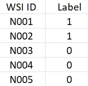
Step 3: Label preprocessing. This step involves selecting, cleaning, and encoding the clinicopathological characteristics. The main idea is to create a table with at least 2 columns. The first column is the slide ID (or the name of WSI) and the second column is the label.
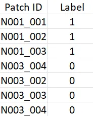
For single-instance learning, every patch that is sampled from a WSI has the label of the root WSI. We can create a modified version of the table with “Patch ID” (instead of “Slide ID”) and “Label” columns.
Step 4: Data Loading. In this step, we construct a data object that loads the patches (from the patch root folder) and their corresponding labels (from the label table) into the same programming environment. Pytorch and TensorFlow have functions or objects to support data loading. Here is my handmade code snippet to illustrate how to construct a data loader in Pytorch:
import os
import torch
import pandas as pd
from PIL import Image
import torchvision.transforms as t
from torch.utils.data import Dataset, DataLoader

class MyData(Dataset):

  def __init__(self, patch_path, label_path, preprocess=None):
"""
patch_path: the path to the folder containing cropped patches from all the root WSIs
label_path: the path to the csv file label table
"""

  self.patches, self.labels, self.ID = [], [], []

  if preprocess is None:
    self.preprocess = t.Compose([
      t.ToTensor(),
      t.Normalize(
        [0.5]*3,
        [0.5]*3
      )
  else:
    self.preprocess = preprocess

  data = pd.read_csv(label_path)
  IDs = list(data["Patch ID"])
  labels = list(data["Label"])

  for p in os.listdir(patch_path):
    patch_name = p[:-4]
    idx = IDs.index(patch_name)

    patch = os.path.join(patch_path, p)
    label = labels[idx]
    ID = IDs[idx]

    self.ID.append(ID)
    self.patches.append(patch)
    self.labels.append(label)

  def __getitem__(self, idx):
    ID, patch, label = self.ID[idx], self.patches[idx], self.labels[idx]

    patch = Image.open(patch).convert("RGB")
    patch = self.preprocess(patch)

    return ID, patch, label

data = MyData(patch_path=patch_path, label_path=label_path, preprocess=None)
loader = DataLoader(data, batch_size=32, shuffle=True)

for batch in loader:
  ID, patch, label = batch[0], batch[1], batch[2]
Step 5: Constructing Training Pipeline. This step is similar to classic deep-learning tasks. The details of the training process, including loss function, epochs, learning rate, data augmentations, and so on, depend on the task at hand. We will not dive into the details of this process because it is well written in somewhere else.
Conclusion
The data structure of histopathology computer vision tasks consists of histopathologic slides and clinicopathological metadata. The main difference between histopathology and classic computer vision deep learning tasks lies in the data preparation steps.