Multiple Instance Learning (MIL) and its utility in Whole Slide Image (WSI) analyses

Introduction
In this discussion, we will attempt to address these 3 bullet questions:
-
What is Multiple Instance Learning (MIL)?
-
Why is MIL conceptually so appropriate for WSI analyses?
-
How does MIL work in WSI analyses?
Definition
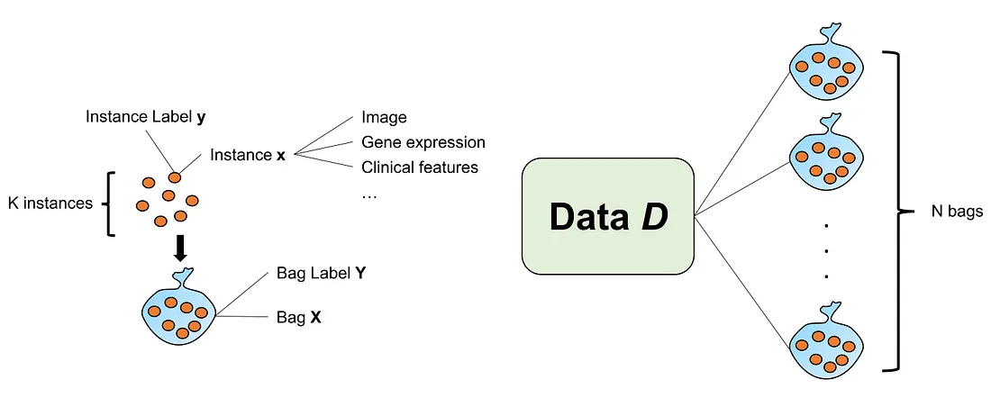
Multiple Instance Learning (MIL) is a type of supervised learning where a group of instances (such as images) is labeled without individual instance labeling. MIL is also a type of weakly supervised learning because not every individual instance is actually labeled. In MIL terms, a group of related instances for one label is called a bag.
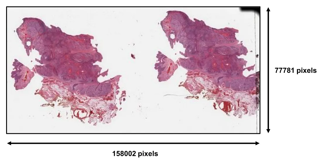
A whole slide image (WSI) is a large, gigapixel, and super-resolution image, that is not easily used as a single input for computer vision models (CVMs), including both convolutional neural networks (CNNs) and vision transformers (ViT).
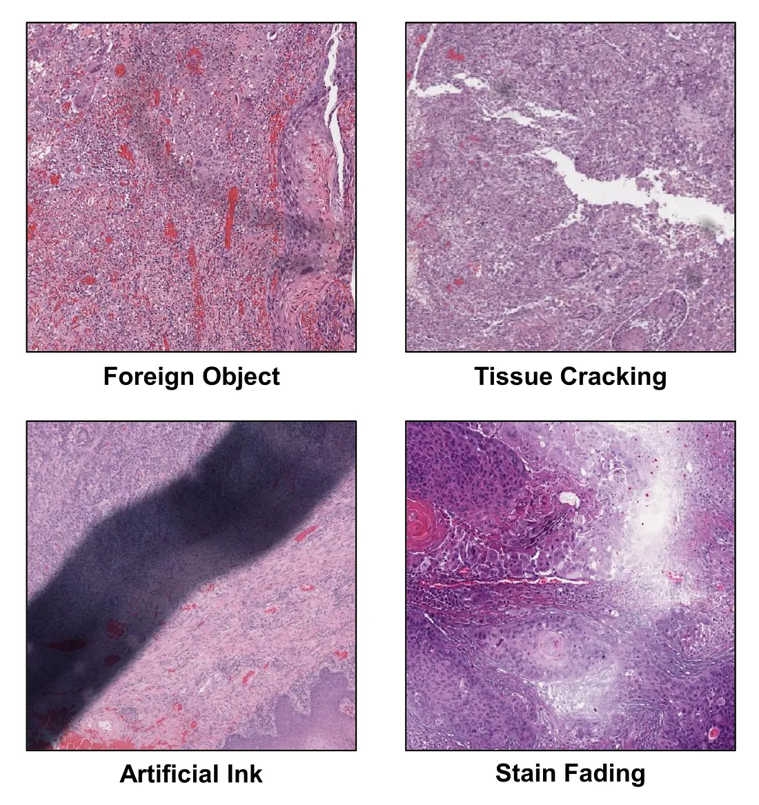
 The WSI is the level of visual information that pathologists deal with in each clinical case. Several important morphologic characteristics are drawn from distinct areas of the WSI. Therefore, a full evaluation of WSI requires the pathologist to scan and look for key features throughout the WSI. To perform an equivalent task, the obvious solution is to train a CVM that takes WSI as an input and predicts the output. However, this approach is quite challenging in reality, given the fact that WSI is too large for an in-house graphical processing unit (GPU) to handle and there are actually many different types of tissue-processing and man-made artifacts in the WSI, which potentially dampens the model’s performance. Additionally, information redundancy also happens. For example, we may encounter a lot of areas with the same information such as the same tumor growth patterns or the same invasive patterns. Such cases are not very rare.
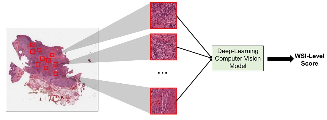
 This is where MIL comes in handy. We can consider a WSI as a bag and each smaller and regional image (patch) of the WSI as an instance. In MIL, the WSI can be cropped into several patches and such patches are then input into the MIL framework to yield the corresponding final WSI-level score.
 If we properly design the framework, MIL can (1) reduce the input size; (2) potentially avoid artifacts; (3) reduce data redundancy; and (4) provide more room for model improvement. Before we discuss the MIL framework in WSI analyses (MIL-WSI), we will explore the problem statement of MIL.
Problem Statement of general MIL (MIL-G)
 Although the problem statement of MIL-G is somewhat different from MIL-WSI, it should be mentioned and distinguished from that of MIL-WSI.
Provide that we have a data D that is arranged in bags {X} and bag labels {Y}. Considering a given bag X, we have k instances inside the bag X={x1, …, xk}. Similarly, we have corresponding k instance labels inside the bag label Y={y1,…,yk}. If there exists an instance label yi=1, then Y=1. Vice versa, if all y1, …, yk=0, then Y=0.
Refined Problem Statement of MIL-WSI
From now on, I will replace the word “bag” with “WSI” and the word “instance” with “patch”, which helps us get used to the context of MIL-WSI.
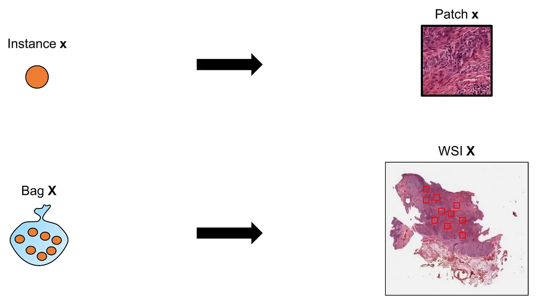 Provide that we have a data D that is arranged in WSIs {X} and WSI-level labels {Y}. Considering a given WSI X, we create k patches inside the WSI X={x1,…xk}. We do not know whether there exist k patch “hard” labels in reality. Patch “hard” label is not a natural concept in many situations of MIL-WSI and, therefore, may not be appropriate to use as a generalized term. Instead, we would want to investigate the patch “soft” labels, or patch contribution, to the final WSI-level label.
Main Components of MIL-WSI Framework
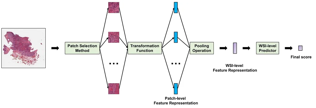 MIL frameworks have a similar overall structure. The detail of each component, of course, varies tremendously from case to case. To help us discuss the MIL framework more easily, I will break it into 4 main components, including:
(i) A patch selection method dictates the mechanisms of how the histopathological patches are selected from a WSI.
(ii) A transformation function f(x) converting a histopathological image into a lower morphologic representation. f(x) is basically a CVM that converts a patch into a patch-level feature representation, which can be a multi-dimensional vector (lower dimensions than the patch) or a score (1-dimensional vector).
(iii) A pooling operation that aggregates the patch-level feature representations of a WSI into a single WSI-level feature representation.
(iv) A WSI-level predictor g(X) that converts the WSI-level representation into the final score.
In histopathology computer vision, the transformation function is usually a computer vision model, such as a CNN or ViT. The WSI-level predictor is usually a multi-layer perceptron (MLP) transforming the WSI-level feature representation into the final score. These 2 components are actively investigated by the research community. In this mini-review, we will focus on the patch selection method and pooling operation.
Categories of Patch Selection Methods
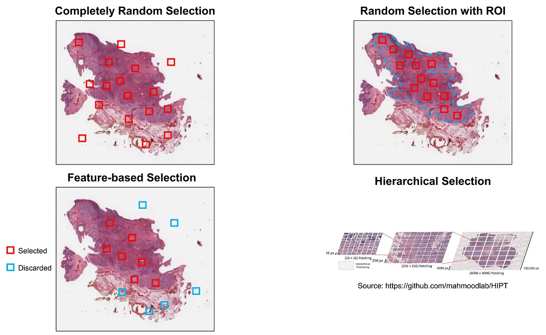
In patch selection, we try to develop a way to select the set of patches as informative as possible to represent the WSI. The options for selecting the patches range from simple to complicated and algorithmic manners, as follows:
(i) Completely random selection. This is the simplest and usually the first choice in MIL, but it is usually not a great idea in MIL-WSI from my experience. While this method can reduce the computation cost, it does not avoid the artifacts. Artifact-containing patches can still be accidentally selected in a random process.
(ii) Random selection with the region of interest (ROI). This is also a simple way to select the patches. The ROIs are manually annotated by pathologists to avoid artifacts and uninformative areas (space, hemorrhage, etc.). This category can reduce the computation cost, avoid artifacts, and select relatively informative patches. The drawback of this method is that it requires human (pathologist/expert) effort to annotate the slide.
(iii) Feature-based selection. An example is to use K-means clustering on patch-level feature representation [1]. Another example of this category is Multiple Instance Learning via Embedded Structures with Local Feature Selection (MILES-LFS) [2].
(iv) Hierarchical selection. This is a special type where a WSI is divided into regional grids, which, in turn, are cut into subregional patches (patching). We can further divide subregional patches into patches. This method is described in Hierarchical Image Pyramid Transformer (HIPT) [3]. The main idea is not to reduce the WSI dimensions but to partition it and convert smaller patches into feature representations.
 Finally, we can also combine these methods together. For example, we first select the patch with ROI and then perform feature selection in the ROI-selected patches.
Categories of Pooling Operations
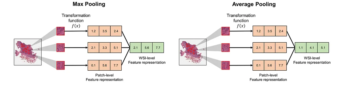
In the pooling operation, we try to attribute the importance of each patch-level representation to effectively create a good WSI-level feature representation. In my experience, pooling operations can be broadly divided into the following 2 categories:
Static Pooling: these operations make a definitive choice about which patches to consider when making a prediction for a WSI. The important characteristic of this category is that these operations do not change as the training process goes on. Examples include max pooling and average pooling.
 Adaptive Pooling: These methods adaptively update the patch contribution to its WSI. This category contains trainable pooling, dynamic pooling, differential evolutionary pooling, and so on. Generally, the adaptive pooling operation is changed iteration by iteration as we train the MIL-WSI framework. Interesting examples of this category are Attention-based pooling [4] and Hopfield pooling [5], both of which belong to trainable pooling.
Conclusion
We conclude this discussion by providing brief answers to the bullet questions.
- What is Multiple Instance Learning (MIL)?
MIL is a type of supervised learning where a set of patches is used to predict a single WSI-level label.
- Why is MIL conceptually so appropriate for WSI analyses?
Each WSI can be considered as a bag while each patch can be regarded as an instance. MIL can (1) reduce the input size; (2) potentially avoid artifacts; (3) reduce data redundancy; and (4) provide more room for model improvement.
- How does MIL work in WSI analyses?
Patches are first selected by a patch selection method and converted into patch-level feature representations by a transformation function. Such patch-level feature representations are aggregated by a pooling operation and converted into the final score by a WSI-level predictor.
To those who may be interested, I hope you enjoy this mini-review.
References
-
Yao, Jiawen, et al. “Whole Slide Images Based Cancer Survival Prediction Using Attention Guided Deep Multiple Instance Learning Networks.” Medical Image Analysis, vol. 65, Oct. 2020, p. 101789, https://doi.org/10.1016/j.media.2020.101789. Accessed 11 June 2021.
-
Shahrjooihaghighi, Aliasghar, and Hichem Frigui. “Local Feature Selection for Multiple Instance Learning.” Journal of Intelligent Information Systems, 1 Nov. 2021, https://doi.org/10.1007/s10844-021-00680-7. Accessed 30 May 2022.
-
Chen, Richard J., et al. “Scaling Vision Transformers to Gigapixel Images via Hierarchical Self-Supervised Learning.” ArXiv:2206.02647 [Cs], 6 June 2022, arxiv.org/abs/2206.02647.
-
Ilse, Maximilian, et al. “Attention-Based Deep Multiple Instance Learning.” ArXiv.org, 28 June 2018, arxiv.org/abs/1802.04712.
-
Ramsauer, Hubert, et al. “Hopfield Networks Is All You Need.” ArXiv:2008.02217 [Cs, Stat], 28 Apr. 2021, arxiv.org/abs/2008.02217.