My Experience in Survival Prediction of Histopathology-based Computer Vision Models
Introduction
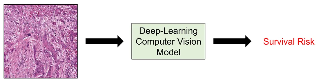
When it comes to medical research, one of the most important aspects is survival risk. A clinical or pathological factor will be noticed if it is associated with a better or worse prognosis. Moreover, when the number of studies as well as our knowledge about this factor increases, it can be a contributor to the management or therapeutical modalities of patients. The survival risk, or prognosis, itself can be measured by many metrics, including overall survival, disease-specific survival, disease-free survival, recurrence-free survival, metastasis-free survival (if the disease of interest is cancer), and so on.
In computer vision, I noticed survival prediction is not a very common task compared to regression, classification, segmentation, etc. while the task of modeling survival risk is more common in machine learning (ML). ML models predicting prognosis consist of the Proportional Hazard Cox Regression Model and Survival Random Forest. Of course, these models and their variants are just a few examples. However, the problem with ML models is that they utilize structured data, meaning tabular data with numeric or categorical features, which is not visual information.
Herein, I summarize some of the common approaches to performing survival prediction in computer vision for histopathology from my experience. First, we will go through some common approaches. I divided these approaches into 3 main categories as follows: (1) transfer learning with downstream ML survival models; (2) transforming into classification task; and (3) employing survival-specific loss function. Then, we will conclude the discussion by briefly mentioning the multiple-instance learning and why it is so appropriate for survival prediction in histopathology computer vision.
Approach 1: Transfer learning with downstream ML survival models
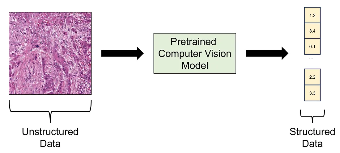
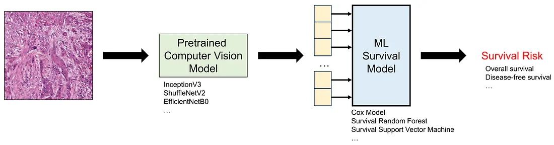 Transfer learning is the term where you employ a pretrained deep learning model to perform the task at hand. The pretrained model is a model that is already trained in a public dataset like ImageNet-1K, meaning that you do not necessarily train the model again. In this approach, we can think of the pretrained model as a data converter since it takes an image, which is unstructured data, as the input and yields a numerical vector as the output, which is structured data.
After converting all the histopathological images into numerical vectors, we can easily train the ML survival models based on these numerical features. Of course, we also need to perform cross-validation, train-test split, or external testing, to ensure the framework (pretrained model + downstream ML survival model) works well as casually.
Approach 2: Transforming into a classification task
 In this approach, we would like to transform the survival data (or censored data) into a categorical variable. In order to understand more about this transformation, we need to understand the basic form of survival data. The survival “variable” is a mixed feature, containing 2 different variables, namely follow-up time (positively continuous) and censoring status (categorical or ordinal).
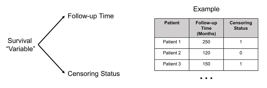
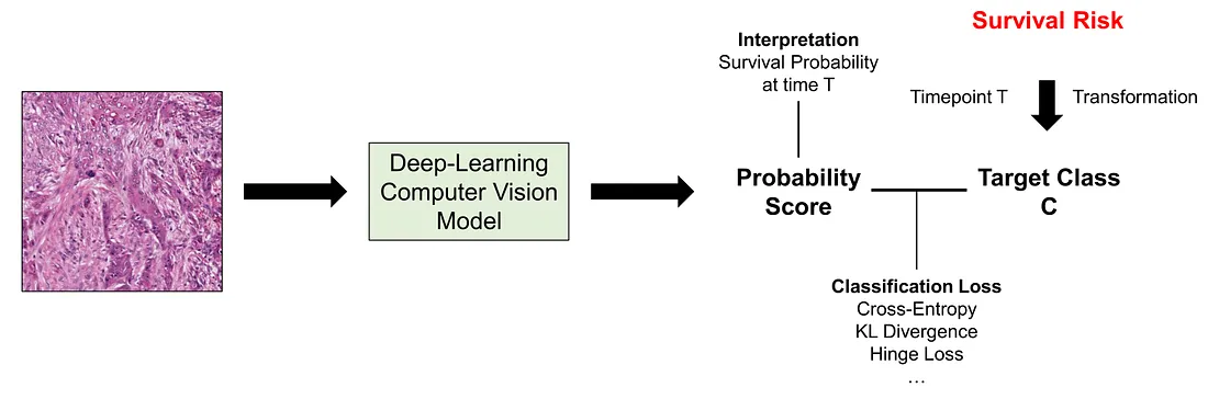
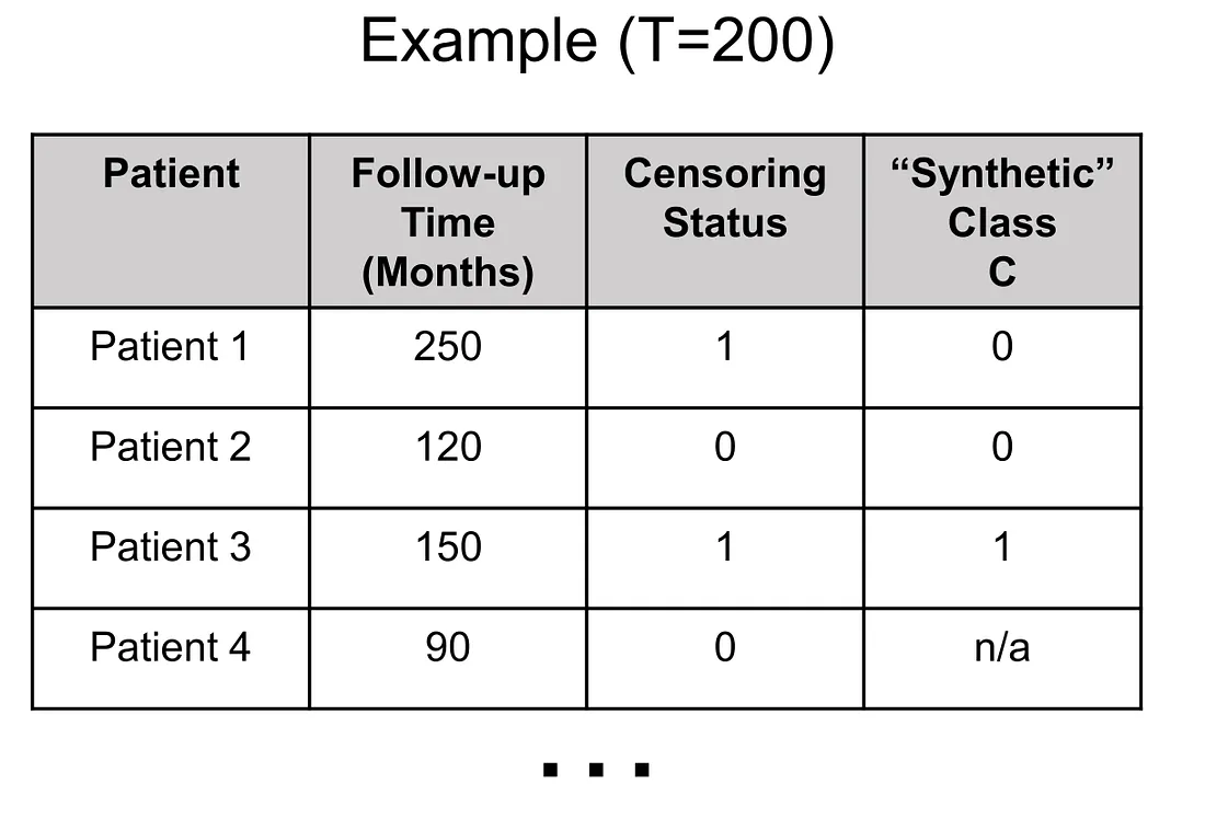
In survival-classification transformation, the first thing to do is to choose the time point (T) where we find it of most importance in the clinical situation although there are several factors we have to consider as well. We will get back to the time point determination later. Secondly, we create the classification task C by the following rules:
(1) Given a patient, if follow-up time > T, then C = 0
(2) Given a patient, if follow-up time ≤ T and censoring status = 0 (no event), then C cannot be determined (C = n/a)
(3) Given a patient, if follow-up time ≤ T and censoring status = 1 (event happened), then C = 1
Applying these rules, the values of synthetic variable C in patients 1, 2, and 3 are 0, 0, 1. Also, I added another patient to illustrate when we encounter the “n/a” value of C.
Of course, the survival data can be much more complicated when we have different events (events 1, …, m). The C variable should be multi-class (m-class variable) in this case. Not to mention we may have different Ts for each of the events, which adds another dimension to the complexity of this transformation procedure.
Understanding the whole picture of this transformation, we know that the determination of T does not only take clinical importance but also class balance and class availability into account. For example, if you choose too large T, you will get a lot of “C=n/a” values because most of the patients are not in follow-up that long. You will also get a lot of “C=1” with a large T since the longer the time of follow-up, the more likely the event will happen. On the other hand, a smaller T value creates a lot of “0” value of C.
Going back to the original problem, the survival-classification transformation provides us with a classification task (C variable), which is one of the most common tasks in computer vision. We can casually use cross-entropy loss or other classification loss to train our model. Naturally, the output of the model will be the survival probability of the patient at the time T.
Approach 3: Employing Survival-Specific Loss Function
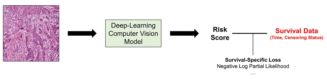 In this approach, we use the survival “variable” itself as the target (unlike approach 2) and directly adjust the computer vision models via backpropagation (unlike approach 1). While one may think that this approach seems the most natural one, it requires a profound understanding of the statistics of survival analysis to design the function and interpret the results. The choice of the most effective loss function for survival tasks is a subject of debate and is often less definitive than in classification tasks. I will mention a few of the loss functions for survival tasks without diving into the details.
Negative Log Partial Likelihood Function: the log partial likelihood function dates back to Sir David Cox himself. This is basically the function we use in fitting the Cox proportional hazard regression model.
Combination of Ordinal Regression Losses and Discordant Loss: this loss consists of ordinal regression loss, truncated ordinal regression loss, and discordant loss. The idea of this combined loss is to maximize and minimize predicted survival probability before and after the time of the event, respectively.
There are many other loss functions that I am not familiar with. Of course, I will continue my learning about these functions.
Conclusion
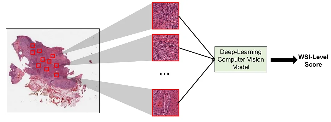
Another interesting fact is that a single histopathological image (1024 x 1024 pixels, for example), as we pathologists know, can not fully describe the whole landscape of pathological lesions. This is where multiple-instance learning (MIL) comes in handy. MIL is a type of supervised learning where a group of instances (such as images) is labeled without individual instance labeling. This is particularly true for histopathological whole slide images (WSIs) and survival tasks since survival data is patient-level information. In other words, we cannot say each image has its prognosis but rather say the constellation of histopathological images representing the patient, has its prognosis. However, we will not be diving too much into MIL since it is another entire topic.
In summary, scientists have developed several approaches to overcome the optimization challenge of survival tasks in histopathology computer vision. The choice to use which approach, again, depends on the task at hand. There is no one-size-fits-all option at this moment.
To those who may be interested, I hope you enjoy this mini-review about this topic.