Data Simulation is a helpful tool for learning Bioinformatics

As a self-study beginner, I understand how challenging it can be to put the first bricks to build bioinformatic skills, especially the eagerness to master the codes necessary for running real analyses. However, the path from the starting point to the moment of actual implementation is long and can be somewhat frustrating.

Image by DALL-E 3 prompted by Author

In this blog, I aim to provide code simulations to assist learners in understanding how to run a few basic bioinformatic pipelines in R. These include RNA sequencing, DNA methylation, single-cell RNA sequencing, and spatial transcriptome.

The main benefit of this simulation approach is that there’s no need to download data, a process that often requires significant time and effort and is prone to errors. This way, beginners can focus on the crucial aspects of data analysis and visualization within these pipelines.

Another cool thing is that beginners can understand the data structure or shape by examining the codes of simulation. This will be helpful when we prepare the real data for our research projects.

Preparation

Things we need to prepare before diving into codes:

• About 5GB space free
• Installing packages
• Creating appropriate directory

Let us prepare the necessary packages for this tutorial blog. If you’ve already installed these packages, there’s no need to run the following code as it could be time-consuming. However, if you only need a few packages, feel free to install them individually. Please note that running this code could take some time, ranging from several minutes to an hour:

general_packages = c("ggplot2", "gridExtra", "dplyr", "tidyverse", 
                      "BiocManager", "readr", "writexl")
bioc_packages = c("org.Hs.eg.db", "DESeq2", "fgsea", 
                  "GSVA", "ChAMP", "Seurat",
                  "IlluminaHumanMethylation450kanno.ilmn12.hg19",
                  "IlluminaHumanMethylationEPICanno.ilm10b4.hg19",
                  "SpotClean")

lapply(general_packages, install.packages, character.only=TRUE)
lapply(bioc_packages, BiocManager::install, character.only=TRUE)

We have to make sure these packages are properly installed for subsequent analyses. Yet, these packages are important for our simulated data analyses as well as future real data analyses.

Once the packages are installed, we need to set up a directory to ensure our work is organized and easily accessible.

• Firstly, create an empty R script named simulation.R.
• Then, place the simulation.R file in a folder that is both visible and convenient for you.
• Exit RStudio and then restart it by opening the simulation.R script. This action sets the working directory to the location of the simulation.R file.

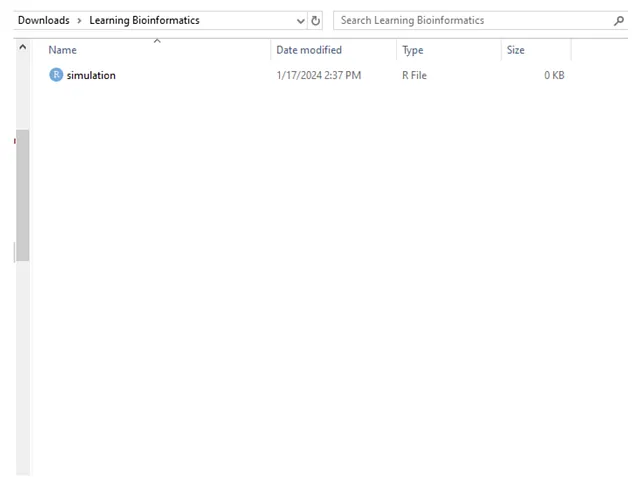
Image by Author

root = paste0(getwd(), "/simulated_blog")
rnaseq_root = paste0(getwd(), "/simulated_blog/RNAseq")
methylation_root = paste0(getwd(), "/simulated_blog/methylation")
scrnaseq_root = paste0(getwd(), "/simulated_blog/ScRNA")
ST_root = paste0(getwd(), "/simulated_blog/ST")

# Create the directories
dir.create(root)
dir.create(rnaseq_root)
dir.create(methylation_root)
dir.create(scrnaseq_root)
dir.create(ST_root)

After running this code block, we will get the folder like this:

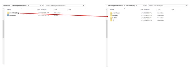
Image by Author

RNA-seq Simulation and Analysis

Here is the simulation code:

setwd(rnaseq_root)
library(org.Hs.eg.db)

set.seed(1)
# Define genes
Genes = keys(org.Hs.eg.db, keytype="SYMBOL")
Genes = Genes[!duplicated(Genes)]
n_genes = length(Genes)

# Define samples
n_samples = 50
Samples = paste0("S", 1:n_samples)

# Assume 2 real phenotypes: A and B
real_phenotype = c(rep("A", n_samples/2), rep("B", n_samples/2))

# Count matrix simulation
nA = n_samples/2 ; nB = n_samples/2
countData = matrix(0, nrow=n_genes, ncol=n_samples)

pb = txtProgressBar(min=0, max=n_genes, initial=0, style=3)

for (i in 1:n_genes){
  sizeA = round(runif(1, 1, 500))
  sizeB = round(runif(1, 1, 500))
  probA = runif(1)
  probB = runif(1)
  readcountA = rnbinom(n=nA, size=sizeA, prob=probA)
  readcountB = rnbinom(n=nB, size=sizeB, prob=probB)
  readcount = c(readcountA, readcountB)
  countData[i,] = readcount
  setTxtProgressBar(pb, i)
}

rownames(countData) = Genes
colnames(countData) = Samples

# Simulate phenotypes in reality
HistologyA = sample(c("H1", "H2"), size=nA, prob=c(0.8, 0.2), replace=TRUE)
HistologyB = sample(c("H1", "H2"), size=nB, prob=c(0.7, 0.3), replace=TRUE)
Histology = c(HistologyA, HistologyB)

MolecularA = sample(c("M1", "M2"), size=nA, prob=c(0.6, 0.4), replace=TRUE)
MolecularB = sample(c("M1", "M2"), size=nA, prob=c(0.1, 0.9), replace=TRUE)
Molecular = c(MolecularA, MolecularB)

colData = data.frame(Histology, Molecular)

The final outputs of this code are countData and colData, which represent the count matrix and the phenotype metadata, respectively. In this code, I’ve constructed a for loop to generate distinct negative binomial distributions between phenotype A and phenotype B for any given gene. The goal is to create two unique biological clusters associated with these phenotypes. Additionally, I’ve created real-world phenotypes, including Histology and Molecular. These have been intentionally designed with a degree of noise, as real-world data is seldom perfect.

This is how the countData and colData look like:

> print(countData[1:5, 1:5])
        S1   S2   S3   S4   S5
A1BG    95   90  111   88   90
A2M    427  451  407  401  407
A2MP1  299  305  297  341  266
NAT1  1135 1286 1409 1149 1199
NAT2   462  421  409  404  385


> print(colData[1:5,])
   Histology Molecular
S1        H1        M1
S2        H1        M2
S3        H1        M2
S4        H1        M1
S5        H1        M2

In countData, each column corresponds to a sample and each row corresponds to a gene. The values represent the expression level of a particular gene in a specific sample. In colData, each column represents a real-world phenotype. The order of the rows in colData matches the order of the columns in countData, indicating that they correspond to the same sample.

We can then proceed with the differential expression analysis. For this purpose, I utilize DESeq2:

library(DESeq2)

# Input of DESeq2: countData, colData

# If we want to compare M1 and M2 of molecular phenotype:
dds = DESeqDataSetFromMatrix(countData=countData, colData=colData, design=~Molecular)

# Run DESeq2
dds = DESeq(dds)
res = results(dds)
print(res)

# Additional: how to save the results
library(readr)
library(writexl)

Gene = rownames(res)
final_res = as.data.frame(cbind(Gene, res))

# If we want to save csv file
write_csv(final_res, "DESeq2_results_Molecular.csv")
# If we want to save xlsx file
write_xlsx(final_res, "DESeq2_results_Molecular.xlsx") 

Next, we conduct pathway analysis. In this instance, I employ the Gene Set Enrichment Analysis (GSEA):

library(msigdbr)
library(fgsea)
library(dplyr)
library(tidyverse)
library(tidyr)

# Define the pathway
# I will use "H" collection in MSigDB database
H = msigdbr(species="Homo sapiens", category="H")
pathways = H %>% group_by(gs_name) %>%
    summarise(pathways=list(gene_symbol)) %>%
    unique() %>%
    deframe()
# list of pathways is the format fgsea uses

# Define the metrics
# In this case I use the metric from the DESeq2 result
stats = res$stat
names(stats) = rownames(res)

# Run GSEA
gsea_res = fgsea(pathways=pathways, stats=stats)


# Additional: how to save the results
library(readr)
library(writexl)

# If we want to save csv file
write_csv(final_res, "GSEA_results_Molecular.csv")
# If we want to save xlsx file
write_xlsx(final_res, "GSEA_results_Molecular.xlsx") 

The gsea_res object encompasses all the computed statistics from the conventional GSEA. An explanation of these terms is beyond the scope of this blog.

Lastly, we can investigate the heterogeneity of pathway activity by conducting single-sample GSEA. For this, I utilize the Gene Set Variational Analysis (GSVA):

library(msigdbr)
library(GSVA)
library(dplyr)
library(tidyverse)
library(tidyr)

# Define the pathway
# I will use "H" collection in MSigDB database
H = msigdbr(species="Homo sapiens", category="H")
pathways = H %>% group_by(gs_name) %>%
    summarise(pathways=list(gene_symbol)) %>%
    unique() %>%
    deframe()
# list of pathways is the format GSVA uses
gsva_res = gsva(expr=countData, gset.idx.list=pathways)
head(gsva_res)

# Additional: how to save the results
library(readr)
library(writexl)

Pathway = rownames(gsva_res)
gsva_res = as.data.frame(c(Pathway, gsva_res))

# If we want to save csv file
write_csv(gsva_res, "GSVA_results_H.csv")
# If we want to save xlsx file
write_xlsx(gsva_res, "GSVA_results_H.xlsx") 

The resulting gsva_res object comprises 50 Pathways x 20 Samples. Each cell contains the enrichment score of a given pathway for a sample.

Upon execution of the codes, the “RNAseq” folder is as follows:

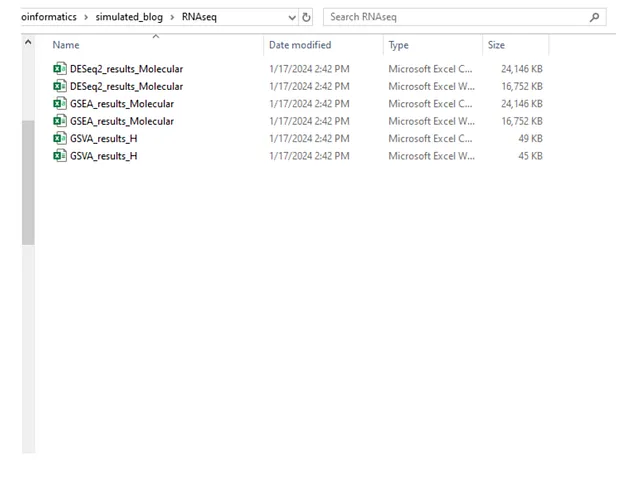
Image by Author

There are numerous other analyses applicable to RNA-seq data. However, they fall outside the purview of this blog.

Methylation Simulation

Here is the simulation code:

setwd(methylation_root)
library(IlluminaHumanMethylation450kanno.ilmn12.hg19)

set.seed(1)
# Define genes
CpGs = IlluminaHumanMethylation450kanno.ilmn12.hg19::Other
CpGs = rownames(CpGs)
n_cpg = length(CpGs)

# Define samples
n_samples = 50
Samples = paste0("S", 1:n_samples)

# Assume 2 real phenotypes: A and B
real_phenotype = c(rep("A", n_samples/2), rep("B", n_samples/2))

# Beta-value matrix simulation
nA = n_samples/2 ; nB = n_samples/2
beta_matrix = matrix(0, nrow=n_cpg, ncol=n_samples)

pb = txtProgressBar(min=0, max=n_cpg, initial=0, style=3)

for (i in 1:n_cpg){
  shape1A = runif(1, 1, 500)
  shape1B = runif(1, 1, 500)
  shape2A = runif(1, 1, 500)
  shape2B = runif(1, 1, 500)
  betaA = rbeta(n=nA, shape1=shape1A, shape2=shape2A)
  betaB = rbeta(n=nB, shape1=shape1B, shape2=shape2B)
  beta = c(betaA, betaB)
  beta_matrix[i,] = beta
  setTxtProgressBar(pb, i)
}

rownames(beta_matrix) = CpGs
colnames(beta_matrix) = Samples

# Simulate phenotypes in reality
HistologyA = sample(c("H1", "H2"), size=nA, prob=c(0.9, 0.1), replace=TRUE)
HistologyB = sample(c("H1", "H2"), size=nB, prob=c(0.1, 0.9), replace=TRUE)
Histology = c(HistologyA, HistologyB)

MolecularA = sample(c("M1", "M2"), size=nA, prob=c(0.8, 0.2), replace=TRUE)
MolecularB = sample(c("M1", "M2"), size=nA, prob=c(0.1, 0.9), replace=TRUE)
Molecular = c(MolecularA, MolecularB)

In this code, I’ve constructed a for loop to generate varying methylation distributions between phenotype A and phenotype B. The goal is to create two distinct biological clusters associated with these phenotypes. Similarly to RNA-seq simulation, I’ve created real-world phenotypes, including Histology and Molecular. Currently, I’m utilizing the probes of the Illumina Infinium HumanMethylation450 BeadChip. However, we can easily switch to using the Illumina MethylationEPIC BeadChip probes by simply replacing the CpGs with those related to EPIC.

library(IlluminaHumanMethylationEPICanno.ilm10b4.hg19)
CpGs = IlluminaHumanMethylationEPICanno.ilm10b4.hg19::Other
CpGs = rownames(CpGs)

This is how the beta_matrix looks like:

> print(beta_matrix[1:5, 1:5])
                  S1        S2        S3        S4        S5
cg00050873 0.2958955 0.3261187 0.2963041 0.3303318 0.3372731
cg00212031 0.3100877 0.3247370 0.3113969 0.2962113 0.3145456
cg00213748 0.4729288 0.4960375 0.4759625 0.4660788 0.5242928
cg00214611 0.4066274 0.4113257 0.3547656 0.4055290 0.3877596
cg00455876 0.8325121 0.8565954 0.8418491 0.8520826 0.8732811

In beta_matrix, each column corresponds to a sample and each row corresponds to a CpG position. The values represent the methylation level of a particular CpG position in a specific sample.

I briefly demonstrate the example code of the methylation analysis by using the ChAMP package:

# I recommend to run this code block step by step

library(ChAMP)

myImport = list()
myImport$beta = beta_matrix
myImport$pd = data.frame(Histology, Molecular)
myLoad = champ.filter()

# Quality Control
champ.QC(pheno=myLoad$pd$Histology)
champ.QC(pheno=myLoad$pd$Molecular)

# Data Normalization
myNorm = champ.norm()

# Differential Methylation Position
myDMP = champ.DMP(pheno=myLoad$pd$Histology)
DMP.GUI(pheno=myLoad$pd$Histology)
# myDMP = champ.DMP(pheno=myLoad$pd$Molecular)

# Differential Methylation Region
myDMR = champ.DMR(pheno=myLoad$pd$Histology)
DMR.GUI(pheno=myLoad$pd$Histology)
# myDMR = champ.DMR(pheno=myLoad$pd$Molecular)

# Block analysis
myBlock = champ.Block(pheno=myLoad$pd$Histology)
Block.GUI(pheno=myLoad$pd$Histology)
# myBlock = champ.Block(pheno=myLoad$pd$Molecular)


# GSEA
myGSEA = champ.GSEA(pheno=myLoad$.pd$Histology)
# myGSEA = champ.GSEA(pheno=myLoad$pd$Molecular)


# Additional: how to save the results
library(readr)
library(writexl)

CpG = rownames(myDMP$H1_to_H2)
DMP_output = as.data.frame(cbind(CpG, myDMP$H1_to_H2))
DMR_output = myDMR$BumphunterDMR
Block_output = myBlock$Block
GSEA_output = myGSEA$DMR

# Saving files in .csv format (we can save in .xlsx like previous done)
write_csv(DMP_output, "DMP_results_Histology.csv")
write_csv(DMR_output, "DMR_results_Histology.csv")
write_csv(Block_output, "Block_results_Histology.csv")
write_csv(GSEA_output, "GSEA_results_Histology.csv")

The ChAMP package offers a comprehensive pipeline, ranging from initial to more advanced analyses, including Differential Methylation Position (DMP), Differential Methylation Region (DMR), and GSEA. This package generates numerous intriguing plots during the analysis process, which you’re free to explore.

Upon execution of these codes, the “methylation” folder is as follows:

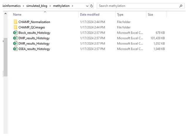
Image by Author

Single-cell RNA-seq Simulation

Here is the simulation code:

setwd(scrnaseq_root)
# Load required libraries
library(Matrix)
library(ggplot2)

# Set the number of genes and cells
library(org.Hs.eg.db)
Genes = keys(org.Hs.eg.db, keytype="SYMBOL")
n_genes = length(Genes)
n_cells = 100
Cells = paste0("Cell", 1:n_cells)
n_CellType = 5
celltypes = c(rep("Fibroblast", n_cells/n_CellType),
              rep("Neutrophil", n_cells/n_CellType),
              rep("Macrophage", n_cells/n_CellType),
              rep("Mast Cell", n_cells/n_CellType),
              rep("Eosinophil", n_cells/n_CellType)
)

# Simulate gene expression data
set.seed(123)
mat <- matrix(0, nrow = n_genes, ncol=n_cells)
pb = txtProgressBar(min=0, max=n_genes, initial=0, style=3)
for (i in 1:n_genes) {
  readcount_fibroblast = rnbinom(n=n_cells/n_CellType, prob=runif(1), size=round(runif(1,1,50)))
  readcount_neutrophil = rnbinom(n=n_cells/n_CellType, prob=runif(1), size=round(runif(1,1,50)))
  readcount_macrophage = rnbinom(n=n_cells/n_CellType, prob=runif(1), size=round(runif(1,1,50)))
  readcount_mastcell = rnbinom(n=n_cells/n_CellType, prob=runif(1), size=round(runif(1,1,50)))
  readcount_eosinophil = rnbinom(n=n_cells/n_CellType, prob=runif(1), size=round(runif(1,1,50)))
  readcount = c(readcount_fibroblast,
                readcount_neutrophil,
                readcount_macrophage,
                readcount_mastcell,
                readcount_eosinophil)
  mat[i,] = readcount
  setTxtProgressBar(pb, i)
}
rownames(mat) = Genes
colnames(mat) = Cells


sparse_mat <- as(mat, "CsparseMatrix")

# Save the data as .mtx file
writeMM(sparse_mat, file = "matrix.mtx")

# Create and save features.tsv.gz and barcodes.tsv.gz files
d = data.frame(feature.names=rownames(mat), gene.column=rownames(mat))


write.table(d, file = "features.tsv", quote = FALSE, row.names = FALSE, col.names = FALSE)
write.table(colnames(mat), file = "barcodes.tsv", quote = FALSE, row.names = FALSE, col.names = FALSE)

# Remove previous data if it exists
if (file.exists("example")){
  unlink("example", recursive = TRUE)
}

# Pack the data
dir_path <- "./example"
library(R.utils)
gzip("matrix.mtx", "example/matrix.mtx.gz")
gzip("features.tsv", "example/features.tsv.gz")
gzip("barcodes.tsv", "example/barcodes.tsv.gz")

In a similar manner, I’ve constructed a for loop to generate varying RNA-seq distributions for, let’s say, 5 different cell types. I’ve also implemented codes to create the real-world objects of scRNA, which are used as input by the Seurat package. These include three compressed files: matrix, features, and barcodes. All these objects are stored in the “example” folder.

I’ve provided an example code for sc-RNA analysis using the Seurat package:

library(Seurat)
data = Read10X(data.dir = "example")
seurat.obj = CreateSeuratObject(counts = data, project="Example")


# Normalize and Scale
seurat.obj = NormalizeData(seurat.obj)
seurat.obj = ScaleData(seurat.obj, features = rownames(seurat.obj))

# Find variable genes
seurat.obj = FindVariableFeatures(seurat.obj)

# Dimension reduction
seurat.obj = RunPCA(seurat.obj, features = VariableFeatures(object = seurat.obj), npcs=10)
seurat.obj = FindNeighbors(seurat.obj, dims = 1:10)
seurat.obj = FindClusters(seurat.obj, resolution = 0.5)
seurat.obj = RunUMAP(seurat.obj, dims = 1:10)
DimPlot(seurat.obj)


# Visualization
# Find 5 most variable genes
features = VariableFeatures(object=seurat.obj)[1:5]

# Which cell cluster has high expression of these genes
FeaturePlot(seurat.obj, features = features)
VlnPlot(seurat.obj, features = features)
RidgePlot(seurat.obj, features = features)
DotPlot(seurat.obj, features = features)
DoHeatmap(seurat.obj, features = features)

The Seurat package is a classic and comprehensive tool that we utilize for sc-RNA data analysis. This package is capable of generating numerous impressive plots.

Upon execution of the codes, the “ScRNA” folder is as follows:

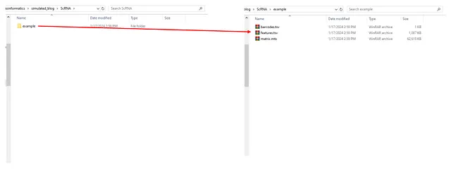
Image by Author

Spatial Transcriptome (ST) Simulation

Here is the simulation code:

SimulateSTData = function(X, Y, n_clusters, tissue, root=getwd()) {
  "
  This function create a simple one-resolutation ST data
  X, Y: width and height of the tissue image
  n_clusters: simulated cluster of transcriptomes
  tissue: list of tissue features, containing: centerX, centerY, radius, shape('I', 'II')
  
  "
  width = X
  height = Y
  n_cells = X * Y
  Cells = paste0("Cell", 1:n_cells)
  
  library(org.Hs.eg.db)
  Genes = keys(org.Hs.eg.db, keytype="SYMBOL")
  Genes = Genes[!duplicated(Genes)]
  n_genes = length(Genes)
  
  # Create tissue mask: a circle with a sin-like border with predefined radius
  mask = matrix(0, nrow=width, ncol=height)
  centerX = tissue$centerX ; centerY = tissue$centerY
  radius = tissue$radius
  a <- 0.6 * radius  # amplitude of the sinusoidal variation
  w <- 2  # frequency of the sinusoidal variation
  
  
  # Define the sinusoidal coefficient function
  sin_coef <- function(x, y) {
    theta <- atan2(y, x)  # angle with the x-axis
    return(a * sin(w * theta))
  }
  
  # Define the circle function
  if (tissue$shape == "I"){
    circle <- function(x, y, r) {
      return(x^2 + y^2 - r^2 - sin_coef(x, y))
    }
  }
  
  
  if (tissue$shape == "II") {
    circle <- function(x, y, r) {
      return((x^2 + y^2 - (r + sin_coef(x, y))^2))
    }
  }
  
  
  for (x in 1:width) {
    for (y in 1:height){
      if (circle(x=(x-centerX), y=(y-centerY), r=radius) <= 0){
        mask[y, x] = 1
      }
    }
  }
  
  
  # Simulate gene expression data
  set.seed(1)
  mat <- matrix(0, nrow = n_genes, ncol=n_cells)
  pb = txtProgressBar(min=0, max=n_genes, initial=0, style=3)
  
  
  for (i in 1:n_genes) {
    readcount = NULL
    for (k in 1:(n_clusters-1)){
      readcount =  c(readcount, rnbinom(n=n_cells/n_clusters, prob=runif(1), size=round(runif(1,1,50))))
    }
    readcount =  c(readcount, rnbinom(n=n_cells-length(readcount), prob=runif(1), size=round(runif(1,1,50))))
    mat[i,] = readcount
    setTxtProgressBar(pb, i)
  }
  rownames(mat) = Genes
  colnames(mat) = Cells
  
  
  # Make sure non-tissue space have no/baseline expression
  for (cell in 1:ncol(mat)){
    x = cell%%height
    y = as.integer(cell/height)
    if (circle(x=(x-centerX), y=(y-centerY), r=radius) > 0){
      mat[,cell] = round(runif(1, 0, 5))
    }
  }
  
  sparse_mat <- as(mat, "CsparseMatrix")
  
  # Create raw folder
  d = data.frame(feature.names=rownames(mat), gene.column=rownames(mat), assay=rep("Expression", nrow(mat)))
  dir_path <- paste0(root, "/raw")
  dir.create(dir_path)
  writeMM(sparse_mat, file = "matrix.mtx")
  write.table(d, file = "features.tsv", quote = FALSE, row.names = FALSE, col.names = FALSE)
  write.table(colnames(mat), file = "barcodes.tsv", quote = FALSE, row.names = FALSE, col.names = FALSE)
  
  library(R.utils)
  gzip("matrix.mtx", paste0(dir_path, "/matrix.mtx.gz"))
  gzip("features.tsv", paste0(dir_path, "/features.tsv.gz"))
  gzip("barcodes.tsv", paste0(dir_path, "/barcodes.tsv.gz"))
  # Create spatial folder
  spatial_dir = paste0(root, "/spatial")
  dir.create(spatial_dir)
  
  # scalefactors_json.json
  json <- list(
    regist_target_img_scalef = 0,
    tissue_hires_scalef = 0,
    tissue_lowres_scalef = 1.0,
    fiducial_diameter_fullres = 0,
    spot_diameter_fullres = 0
  )
  json_data <- toJSON(json, auto_unbox = TRUE)
  write(json_data, file = paste0(spatial_dir, "/scalefactors_json.json"))
  
  library(png)
  library(grid)
  
  # Set the dimensions of the image tissue_lowres_image.png
  width <- Y
  height <- X
  set.seed(1)
  img <- matrix(runif(width * height * 3), nrow = width, ncol = height)
  
  mask
  img = img*mask
  # Reshape the matrix into an array
  img <- array(data = img, dim = c(width, height, 3))
  # Save the image as a .png file
  writePNG(img, paste0(spatial_dir, "/tissue_lowres_image.png"))
  
  # tissue_positions.csv
  in_tissue = NULL ; i = 0
  array_row = rep(seq(0, X-1), Y)
  array_row = array_row[order(array_row)]
  array_col = rep(seq(0, (Y-1), 1), X)
  for (i in 1:length(array_row)) {
    x = array_col[i]
    y = array_row[i]
    if (circle(x=(x-centerX), y=(y-centerY), r=radius) <= 0){
      in_tissue[i] = 1
    } else {
      in_tissue[i] = 0
    } 
  }
  tissue_positions = data.frame(barcode=Cells, in_tissue, array_row, array_col,
                                pxl_row_in_fullres=array_row, pxl_col_in_fullres=array_col)
  write_csv(tissue_positions, paste0(spatial_dir, "/tissue_positions.csv"))
}

Simulating ST data is a complex task. It necessitates an understanding of the spatial correlation among the image, count matrix, barcode, and tissue position metadata. Therefore, I’ve encapsulated the simulation codes into a function for future use. In this simulated data, we treat low-resolution and high-resolution images as having the same size due to memory space constraints. I’ve introduced a “simulated tissue” with an apparently natural shape using a mathematical formula. To add more intrigue, I’ve created two types of tissue shapes.

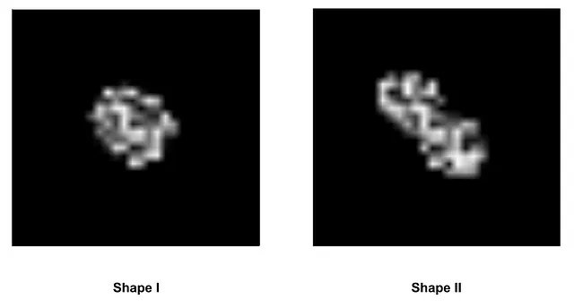
Image by Author

We start using the simulation function:

setwd(ST_root)

library(Matrix)
library(ggplot2)
library(rhdf5)
library(jsonlite)
library(png)
library(SpotClean)
library(readr)
library(Seurat)

# Define parameters
X = 30
Y = 30
n_clusters = 5
tissue = list(centerX = 10, centerY=20, radius=5, shape="I")
root = "STData"

# Remove previous data if it exists
if (file.exists(root)){
  unlink(root, recursive = TRUE)
}

# Simulate ST data
SimulateSTData(X=X, Y=Y, n_clusters=n_clusters, tissue=tissue, root=root)


# Load the data
raw = Read10X("STData/raw")
slide_info = read10xSlide("STData/spatial/tissue_positions.csv",
                                 "STData/spatial/tissue_lowres_image.png",
                                 "STData/spatial/scalefactors_json.json")
ST_obj = createSlide(count_mat = raw,
                         slide_info = slide_info)

The “ST” folder after running the code:

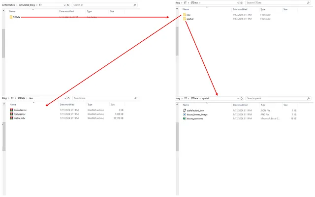
Image by Author

The real-world “STData/spatial” folder contains additional files, such as H&E images and immunofluorescence images. Simulating these images within this blog would be quite cumbersome and not particularly beneficial. To give you an idea, here’s what this folder looks like with real-world data:

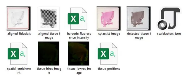
Image by Author

To show the low-resolution original tissue:

visualizeSlide(slide_obj = ST_obj)

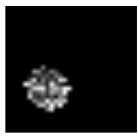
Image by Author

If we want to visualize the spatial expression of a given gene such as TP53. We can use the visualizeHeatmap function like this:

# We use TP53 gene as an example
g = "TP53"
visualizeHeatmap(ST_obj, g)

The image should be:

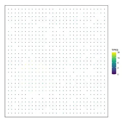
Image by Author

To make it clearer, we could use our customed code with the ggplot2 package:

pd = visualizeHeatmap(ST_obj, g)
pd = pd$data
tmp = expand.grid(row=1:Y, col=1:X)

ggplot(pd) +
  geom_point(data=tmp, aes(x=col, y=-row), size=5, color="grey") +
  geom_point(data=pd, aes(x=col, y=-row, color=value), size=5) +
  scale_color_viridis_c(g)

The resulting image should be:

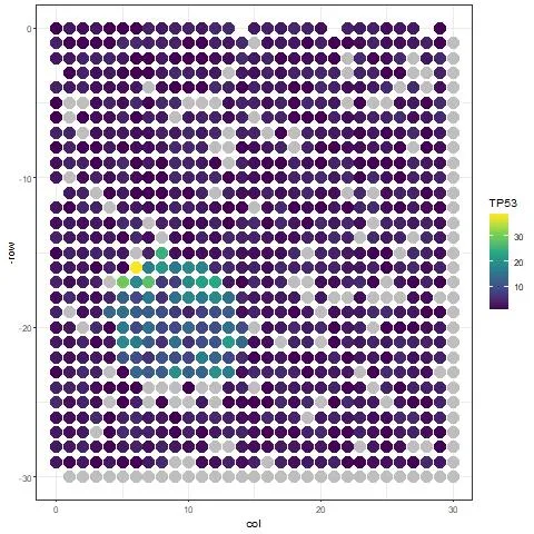
Image by Author

We found that there is too much contamination of expression outside the tissue. The SpotClean package helps us decontaminate the heatmap:

decont_obj = spotclean(ST_obj)

g = "TP53"
pd = visualizeHeatmap(decont_obj, g)
pd = pd$data
tmp = expand.grid(row=1:Y, col=1:X)

ggplot(pd) +
  geom_point(data=tmp, aes(x=col, y=-row), size=5, color="grey") +
  geom_point(data=pd, aes(x=col, y=-row, color=value), size=5) +
  scale_color_viridis_c(g)

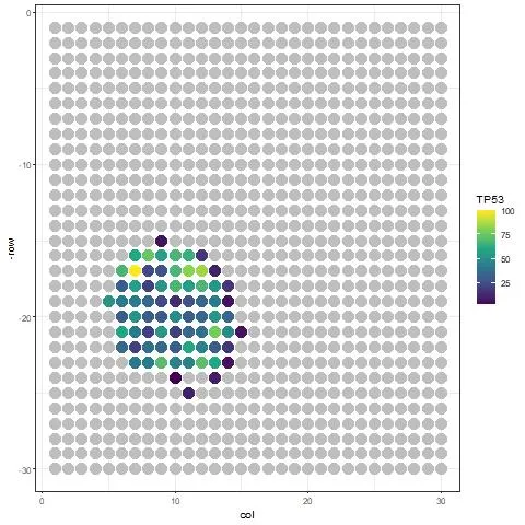
Image by Author

With that, I conclude this blog by creating a combined plot showing the spatial expression of TP53, CCND1, RB1, CTNNB1, EGFR, and IDH1, which are interested genes in cancer research, using this simulated data:

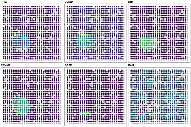
Raw heatmaps - Image by Author

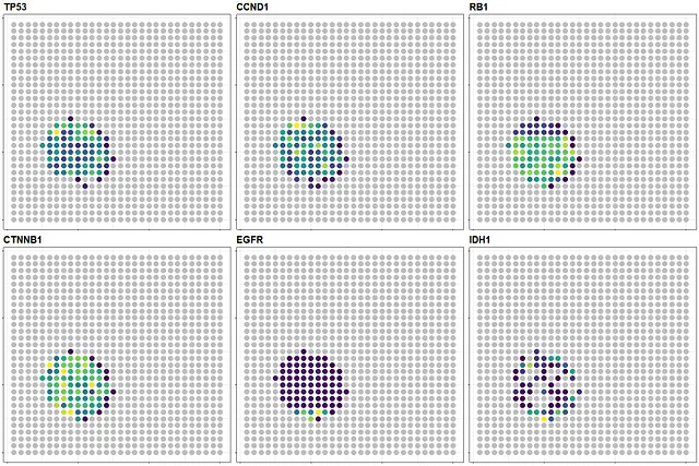
Decontaminated heatmaps - Image by Author

Here is the code I used to generate this plot:

making_fun_plots = function(ST_obj, g){
  pd = visualizeHeatmap(ST_obj, g)
  pd = pd$data
  tmp = expand.grid(row=1:Y, col=1:X)
  p = ggplot(pd) +
    geom_point(data=tmp, aes(x=col, y=-row), size=5, color="grey") +
    geom_point(data=pd, aes(x=col, y=-row, color=value), size=5) +
    scale_color_viridis_c(g) +
    ggtitle(g) +
    theme(legend.position = "none",
          plot.title = element_text(size=20, face="bold"),
          axis.text = element_blank(),
          axis.title = element_blank())
  return(p)
}

# Raw combined plot
p1 = making_fun_plots(ST_obj=ST_obj, g="TP53")
p2 = making_fun_plots(ST_obj=ST_obj,g="CCND1")
p3 = making_fun_plots(ST_obj=ST_obj,g="RB1")
p4 = making_fun_plots(ST_obj=ST_obj,g="CTNNB1")
p5 = making_fun_plots(ST_obj=ST_obj,g="EGFR")
p6 = making_fun_plots(ST_obj=ST_obj,g="IDH1")

gridExtra::grid.arrange(p1, p2, p3,
                        p4, p5, p6,
                        nrow=2)

# Decontaminated combined plot
p1 = making_fun_plots(ST_obj=decont_obj, g="TP53")
p2 = making_fun_plots(ST_obj=decont_obj,g="CCND1")
p3 = making_fun_plots(ST_obj=decont_obj,g="RB1")
p4 = making_fun_plots(ST_obj=decont_obj,g="CTNNB1")
p5 = making_fun_plots(ST_obj=decont_obj,g="EGFR")
p6 = making_fun_plots(ST_obj=decont_obj,g="IDH1")

gridExtra::grid.arrange(p1, p2, p3,
                        p4, p5, p6,
                        nrow=2)

Conclusion

Thank you for taking the time to read this blog. I believe that these simulation codes can serve as valuable tools for learning bioinformatics and understanding the data structure of significant bioinformatic data types.

I welcome any suggestions for improving the provided codes.

---

<

Previous Post

FDPNP4: Artificial Intelligence under the Microscope (Part 3)

>

Next Post

FDPNP5: The operation of neural networks (Part 1)